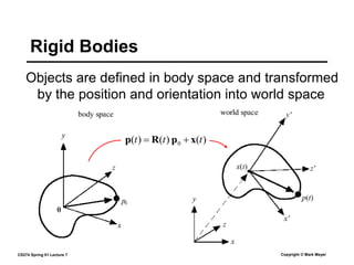
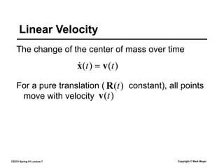
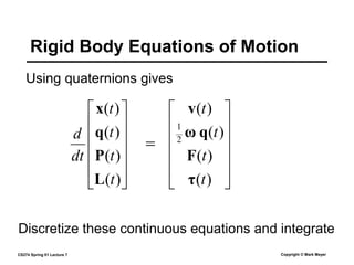
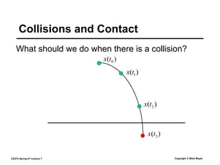
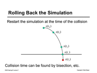
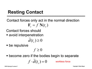
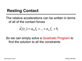
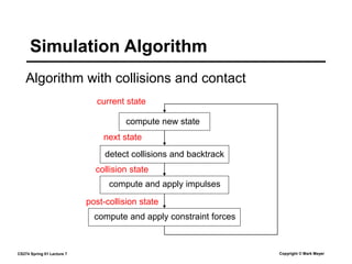
CS274 Spring 01 Lecture 7 Copyright © Mark Meyer
Lecture VII
Rigid Body Dynamics
CS274: Computer Animation and Simulation
CS274 Spring 01 Lecture 7 Copyright © Mark Meyer
Rigid Bodies
Rigid bodies have both a position and orientation
Rigid bodies assume no object deformation
Rigid body motion is represented by 2 parameters
)
(t
x - center of mass
)
(t
R - orientation (rotation matrix)
CS274 Spring 01 Lecture 7 Copyright © Mark Meyer
Rigid Bodies
Objects are defined in body space and transformed
by the position and orientation into world space
)
(
)
(
)
( 0 t
t
t x
p
R
p 

CS274 Spring 01 Lecture 7 Copyright © Mark Meyer
Linear Velocity
The change of the center of mass over time
For a pure translation ( constant), all points
move with velocity
)
(
)
( t
t v
x 

)
(t
v
)
(t
R
CS274 Spring 01 Lecture 7 Copyright © Mark Meyer
Angular Velocity
The change in orientation over time
Encodes both the axis and speed of the rotation
 direction encodes the axis
 magnitude encodes the speed (rad/s)
)
(t
ω
But, how are and related?
)
(t
ω )
(t
R
CS274 Spring 01 Lecture 7 Copyright © Mark Meyer
Angular Velocity
For a given vector
The columns of represent the transformed axes
)
(
)
(
)
( t
t
t r
ω
r 


)
(t
R
)
(
)
(
)
( .
. t
t
t j
j R
ω
R 


1
e
2
e
3
e
1
.
R
2
.
R
3
.
R
ω
r
CS274 Spring 01 Lecture 7 Copyright © Mark Meyer
We can represent the cross product with a matrix
Angular Velocity
b
b
a
b
a 











0
0
0
*
z
y
x
x
y
z
a
a
a
a
a
a
)
(
)
(
)
( *
t
t
t R
ω
R 

Therefore
CS274 Spring 01 Lecture 7 Copyright © Mark Meyer
Since a point can be represented at any time by
Velocity of a Point
Total velocity can then be expressed as
)
(
)
(
)
( 0 t
t
t x
r
R
r 

)
(
)
(
)
( 0 t
t
t v
r
R
r 
 

)
(
)
(
)
( 0
*
t
t
t v
r
R
ω
r 


)
(
))
(
)
(
(
)
( t
t
t
t v
x
r
ω
r 




Which can be rewritten as
CS274 Spring 01 Lecture 7 Copyright © Mark Meyer
We can apply forces to the object at any point
Force

 )
(
)
( t
t i
F
F
Total force on an object is simply
No information about where the forces are applied
)
(
1 t
F
)
(
2 t
F
CS274 Spring 01 Lecture 7 Copyright © Mark Meyer
Torque describes the “rotational force”
Torque

 


 )
(
))
(
)
(
(
)
(
)
( t
t
t
t
t i
i
i F
x
r
τ
τ
Total torque on an object is simply
Tells us about the force distribution over the object
)
(
1 t
F
)
(
2 t
F
)
(
))
(
)
(
(
)
( t
t
t
t i
i
i F
x
r
τ 


)
(t
x )
(
1 t
r
CS274 Spring 01 Lecture 7 Copyright © Mark Meyer
Linear momentum of a particle is
Linear Momentum
Linear momentum of a rigid body is then
v
p m

dV
t
t 
 )
(
)
( r
P 

density
integration over the body
CS274 Spring 01 Lecture 7 Copyright © Mark Meyer
Linear momentum can be simplified as follows
Linear Momentum
dV
t
t 
 )
(
)
( r
P 

dV
t
t
t
t  


 ))
(
)
(
(
)
(
)
( x
r
ω
v
P 

)
(
)
( t
M
t v
P 
Assuming constant mass gives
)
(
)
( t
t F
P 

)
(
)
( t
M
t v
P 
 
CS274 Spring 01 Lecture 7 Copyright © Mark Meyer
Angular momentum of a rigid body
Angular Momentum
)
(
)
(
)
( t
t
t ω
I
L 
Taking the time derivative
)
(
)
( t
t τ
L 

inertia tensor
Angular momentum is conserved for no torque
CS274 Spring 01 Lecture 7 Copyright © Mark Meyer
Describes how mass is distributed in the body
Inertia Tensor











zz
zy
zx
yz
yy
yx
xz
xy
xx
I
I
I
I
I
I
I
I
I
t)
(
I
dV
z
y
Ixx  
 )
ˆ
ˆ
( 2
2

Analogous to mass in linear velocity
Measures the preferred axis of rotation
Expensive to compute this at every time step
dV
y
x
Ixy 

 )
ˆ
ˆ
(

ss
centerOfMa
x
x
x 

ˆ
CS274 Spring 01 Lecture 7 Copyright © Mark Meyer
Rewrite the tensor as
Inertia Tensor
dV
t
t
t
t
t T
 

 )
)
(
ˆ
)
(
ˆ
)
(
ˆ
)
(
ˆ
(
)
( r
r
Id
r
r
I 
Integrals can now be precomputed
dV
t
t
t T
T
T
 
 ))
(
)
)(
(
(
)
( 0
0
0
0 R
r
r
Id
r
r
R
I 
)
(
)
(
)
( t
t
t T
body R
I
R
I 
dV
t
t
t
t
t T
T
 
 )
)
)
(
(
)
(
)
(
)
)
(
((
)
( 0
0
0
0 r
R
r
R
Id
r
R
r
R
I 
CS274 Spring 01 Lecture 7 Copyright © Mark Meyer
Combining the equations
Rigid Body Equations of Motion












)
(
)
(
)
(
)
(
t
t
t
t
dt
d
L
P
R
x
Discretize these continuous equations and integrate












)
(
)
(
)
(
)
(
*
t
t
t
t
τ
F
R
ω
v

CS274 Spring 01 Lecture 7 Copyright © Mark Meyer
Use quaternions to represent orientation
Using Quaternions







axis
q
)
2
/
sin(
)
2
/
cos(
)
(


t
The update rule is then
)
(
)
(
2
1
)
( t
t
t q
ω
q 

CS274 Spring 01 Lecture 7 Copyright © Mark Meyer
Using quaternions gives
Rigid Body Equations of Motion












)
(
)
(
)
(
)
(
t
t
t
t
dt
d
L
P
q
x
Discretize these continuous equations and integrate












)
(
)
(
)
(
)
(
2
1
t
t
t
t
τ
F
q
ω
v

CS274 Spring 01 Lecture 7 Copyright © Mark Meyer
So far, no interaction between rigid bodies
Collisions and Contact
Collision detection –
determining if, when and where a collision occurs
Collision response –
calculating the state (velocity, …) after the collision
CS274 Spring 01 Lecture 7 Copyright © Mark Meyer
)
( 3
t
x
)
( 2
t
x
What should we do when there is a collision?
Collisions and Contact
)
( 0
t
x
)
( 1
t
x
CS274 Spring 01 Lecture 7 Copyright © Mark Meyer
Restart the simulation at the time of the collision
Rolling Back the Simulation
Collision time can be found by bisection, etc.
)
( 3
t
x
)
( 2
t
x
)
( 0
t
x
)
( 1
t
x
)
( c
t
x
CS274 Spring 01 Lecture 7 Copyright © Mark Meyer
Exploit coherency through witnessing
Collision Detection
Speed up with bounding boxes, grids, hierarchies, etc.
separating plane
Two convex objects are
non-penetrating iff there exists a
separating plane between them
First find a separating plane and
see if it is still valid after the next
simulation step
CS274 Spring 01 Lecture 7 Copyright © Mark Meyer
Conditions for collision
Collision Detection
N
A
B
b
a p
p 
 
N
A
B
b
a p
p 
 
N
A
B b
a p
p 
 
))
(
)
(
(
)
(
)
(
)
( t
t
t
t
t a
a
a
a
a x
p
ω
v
p 




0
))
(
)
(
( 

 t
t b
a p
p
N 
 0
))
(
)
(
( 

 t
t b
a p
p
N 
 0
))
(
)
(
( 

 t
t b
a p
p
N 

separating contact colliding
CS274 Spring 01 Lecture 7 Copyright © Mark Meyer
Soft Body Collision
Collision
Force is applied to prevent interpenetration
CS274 Spring 01 Lecture 7 Copyright © Mark Meyer
Soft Body Collision
Collision
Apply forces and change the velocity
CS274 Spring 01 Lecture 7 Copyright © Mark Meyer
Harder Collision
Collision
Higher force over a shorter time
CS274 Spring 01 Lecture 7 Copyright © Mark Meyer
Rigid Body Collision
Collision
Impulsive force produces a discontinuous velocity
CS274 Spring 01 Lecture 7 Copyright © Mark Meyer
We need to change velocity instantaneously
Impulse
Infinite force in an infinitesimal time
t

 F
J
J
P 

M
J
v 

An impulse changes the velocity as
or
CS274 Spring 01 Lecture 7 Copyright © Mark Meyer
An impulse also creates an impulsive torque
Impulse
The impulsive torque changes the angular velocity
J
x
p
τ 

 ))
(
)
(
( t
t
impulse
impulse
τ
L 

impulse
t τ
I
ω )
(
1


 or
CS274 Spring 01 Lecture 7 Copyright © Mark Meyer
For a frictionless collision
Impulse
But how do we calculate ?
N
J j

j
N
A
B
a
J
b
J
CS274 Spring 01 Lecture 7 Copyright © Mark Meyer
For a frictionless collision
Impulse
Given this equation and knowing how affects the
linear and angular velocities of the two bodies,
we can solve for
)))
(
)
(
(
(
))
(
)
(
( t
t
t
t b
a
b
a









 p
p
N
p
p
N 


 
j
j
.̂
.̂
.̂ .̂
CS274 Spring 01 Lecture 7 Copyright © Mark Meyer
Bodies are neither colliding nor separating
Resting Contact
We want a force strong enough to resist
penetration but only enough to maintain contact
CS274 Spring 01 Lecture 7 Copyright © Mark Meyer
We want to prevent interpenetration
Resting Contact
0
))
(
)
(
(
)
( 


 t
t
t
d b
a p
p
N
Since we should keep it from decreasing
0
)
( 
c
t
d
0
))
(
)
(
(
))
(
)
(
(
)
( 





 t
t
t
t
t
d b
a
b
a p
p
N
p
p
N 



Since we should keep it from decreasing
0
)
( 
c
t
d

0
))
(
)
(
(
2
))
(
)
(
(
)
( 





 c
b
c
a
c
b
c
a
c t
t
t
t
t
d p
p
N
p
p
N 








Describes the objects’ acceleration towards one another
CS274 Spring 01 Lecture 7 Copyright © Mark Meyer
Contact forces only act in the normal direction
Resting Contact
Contact forces should
)
( c
c t
f N
F 
0
)
( 
c
t
d

 avoid interpenetration
0

f
 be repulsive
0
)
( 
 c
t
d
f 
 workless force
 become zero if the bodies begin to separate
CS274 Spring 01 Lecture 7 Copyright © Mark Meyer
The relative accelerations can be written in terms
of all of the contact forces
Resting Contact
i
n
n
c
i b
f
a
f
a
t
d 


 ...
)
( 0
0


So we can simply solve a Quadratic Program to
find the solution to all the constraints
CS274 Spring 01 Lecture 7 Copyright © Mark Meyer
Algorithm with collisions and contact
Simulation Algorithm
compute new state
detect collisions and backtrack
compute and apply impulses
compute and apply constraint forces
current state
next state
collision state
post-collision state

rigidBodyDynamics.ppt

  • 1.
    CS274 Spring 01Lecture 7 Copyright © Mark Meyer Lecture VII Rigid Body Dynamics CS274: Computer Animation and Simulation
  • 2.
    CS274 Spring 01Lecture 7 Copyright © Mark Meyer Rigid Bodies Rigid bodies have both a position and orientation Rigid bodies assume no object deformation Rigid body motion is represented by 2 parameters ) (t x - center of mass ) (t R - orientation (rotation matrix)
  • 3.
    CS274 Spring 01Lecture 7 Copyright © Mark Meyer Rigid Bodies Objects are defined in body space and transformed by the position and orientation into world space ) ( ) ( ) ( 0 t t t x p R p  
  • 4.
    CS274 Spring 01Lecture 7 Copyright © Mark Meyer Linear Velocity The change of the center of mass over time For a pure translation ( constant), all points move with velocity ) ( ) ( t t v x   ) (t v ) (t R
  • 5.
    CS274 Spring 01Lecture 7 Copyright © Mark Meyer Angular Velocity The change in orientation over time Encodes both the axis and speed of the rotation  direction encodes the axis  magnitude encodes the speed (rad/s) ) (t ω But, how are and related? ) (t ω ) (t R
  • 6.
    CS274 Spring 01Lecture 7 Copyright © Mark Meyer Angular Velocity For a given vector The columns of represent the transformed axes ) ( ) ( ) ( t t t r ω r    ) (t R ) ( ) ( ) ( . . t t t j j R ω R    1 e 2 e 3 e 1 . R 2 . R 3 . R ω r
  • 7.
    CS274 Spring 01Lecture 7 Copyright © Mark Meyer We can represent the cross product with a matrix Angular Velocity b b a b a             0 0 0 * z y x x y z a a a a a a ) ( ) ( ) ( * t t t R ω R   Therefore
  • 8.
    CS274 Spring 01Lecture 7 Copyright © Mark Meyer Since a point can be represented at any time by Velocity of a Point Total velocity can then be expressed as ) ( ) ( ) ( 0 t t t x r R r   ) ( ) ( ) ( 0 t t t v r R r     ) ( ) ( ) ( 0 * t t t v r R ω r    ) ( )) ( ) ( ( ) ( t t t t v x r ω r      Which can be rewritten as
  • 9.
    CS274 Spring 01Lecture 7 Copyright © Mark Meyer We can apply forces to the object at any point Force   ) ( ) ( t t i F F Total force on an object is simply No information about where the forces are applied ) ( 1 t F ) ( 2 t F
  • 10.
    CS274 Spring 01Lecture 7 Copyright © Mark Meyer Torque describes the “rotational force” Torque       ) ( )) ( ) ( ( ) ( ) ( t t t t t i i i F x r τ τ Total torque on an object is simply Tells us about the force distribution over the object ) ( 1 t F ) ( 2 t F ) ( )) ( ) ( ( ) ( t t t t i i i F x r τ    ) (t x ) ( 1 t r
  • 11.
    CS274 Spring 01Lecture 7 Copyright © Mark Meyer Linear momentum of a particle is Linear Momentum Linear momentum of a rigid body is then v p m  dV t t   ) ( ) ( r P   density integration over the body
  • 12.
    CS274 Spring 01Lecture 7 Copyright © Mark Meyer Linear momentum can be simplified as follows Linear Momentum dV t t   ) ( ) ( r P   dV t t t t      )) ( ) ( ( ) ( ) ( x r ω v P   ) ( ) ( t M t v P  Assuming constant mass gives ) ( ) ( t t F P   ) ( ) ( t M t v P   
  • 13.
    CS274 Spring 01Lecture 7 Copyright © Mark Meyer Angular momentum of a rigid body Angular Momentum ) ( ) ( ) ( t t t ω I L  Taking the time derivative ) ( ) ( t t τ L   inertia tensor Angular momentum is conserved for no torque
  • 14.
    CS274 Spring 01Lecture 7 Copyright © Mark Meyer Describes how mass is distributed in the body Inertia Tensor            zz zy zx yz yy yx xz xy xx I I I I I I I I I t) ( I dV z y Ixx    ) ˆ ˆ ( 2 2  Analogous to mass in linear velocity Measures the preferred axis of rotation Expensive to compute this at every time step dV y x Ixy    ) ˆ ˆ (  ss centerOfMa x x x   ˆ
  • 15.
    CS274 Spring 01Lecture 7 Copyright © Mark Meyer Rewrite the tensor as Inertia Tensor dV t t t t t T     ) ) ( ˆ ) ( ˆ ) ( ˆ ) ( ˆ ( ) ( r r Id r r I  Integrals can now be precomputed dV t t t T T T    )) ( ) )( ( ( ) ( 0 0 0 0 R r r Id r r R I  ) ( ) ( ) ( t t t T body R I R I  dV t t t t t T T    ) ) ) ( ( ) ( ) ( ) ) ( (( ) ( 0 0 0 0 r R r R Id r R r R I 
  • 16.
    CS274 Spring 01Lecture 7 Copyright © Mark Meyer Combining the equations Rigid Body Equations of Motion             ) ( ) ( ) ( ) ( t t t t dt d L P R x Discretize these continuous equations and integrate             ) ( ) ( ) ( ) ( * t t t t τ F R ω v 
  • 17.
    CS274 Spring 01Lecture 7 Copyright © Mark Meyer Use quaternions to represent orientation Using Quaternions        axis q ) 2 / sin( ) 2 / cos( ) (   t The update rule is then ) ( ) ( 2 1 ) ( t t t q ω q  
  • 18.
    CS274 Spring 01Lecture 7 Copyright © Mark Meyer Using quaternions gives Rigid Body Equations of Motion             ) ( ) ( ) ( ) ( t t t t dt d L P q x Discretize these continuous equations and integrate             ) ( ) ( ) ( ) ( 2 1 t t t t τ F q ω v 
  • 19.
    CS274 Spring 01Lecture 7 Copyright © Mark Meyer So far, no interaction between rigid bodies Collisions and Contact Collision detection – determining if, when and where a collision occurs Collision response – calculating the state (velocity, …) after the collision
  • 20.
    CS274 Spring 01Lecture 7 Copyright © Mark Meyer ) ( 3 t x ) ( 2 t x What should we do when there is a collision? Collisions and Contact ) ( 0 t x ) ( 1 t x
  • 21.
    CS274 Spring 01Lecture 7 Copyright © Mark Meyer Restart the simulation at the time of the collision Rolling Back the Simulation Collision time can be found by bisection, etc. ) ( 3 t x ) ( 2 t x ) ( 0 t x ) ( 1 t x ) ( c t x
  • 22.
    CS274 Spring 01Lecture 7 Copyright © Mark Meyer Exploit coherency through witnessing Collision Detection Speed up with bounding boxes, grids, hierarchies, etc. separating plane Two convex objects are non-penetrating iff there exists a separating plane between them First find a separating plane and see if it is still valid after the next simulation step
  • 23.
    CS274 Spring 01Lecture 7 Copyright © Mark Meyer Conditions for collision Collision Detection N A B b a p p    N A B b a p p    N A B b a p p    )) ( ) ( ( ) ( ) ( ) ( t t t t t a a a a a x p ω v p      0 )) ( ) ( (    t t b a p p N   0 )) ( ) ( (    t t b a p p N   0 )) ( ) ( (    t t b a p p N   separating contact colliding
  • 24.
    CS274 Spring 01Lecture 7 Copyright © Mark Meyer Soft Body Collision Collision Force is applied to prevent interpenetration
  • 25.
    CS274 Spring 01Lecture 7 Copyright © Mark Meyer Soft Body Collision Collision Apply forces and change the velocity
  • 26.
    CS274 Spring 01Lecture 7 Copyright © Mark Meyer Harder Collision Collision Higher force over a shorter time
  • 27.
    CS274 Spring 01Lecture 7 Copyright © Mark Meyer Rigid Body Collision Collision Impulsive force produces a discontinuous velocity
  • 28.
    CS274 Spring 01Lecture 7 Copyright © Mark Meyer We need to change velocity instantaneously Impulse Infinite force in an infinitesimal time t   F J J P   M J v   An impulse changes the velocity as or
  • 29.
    CS274 Spring 01Lecture 7 Copyright © Mark Meyer An impulse also creates an impulsive torque Impulse The impulsive torque changes the angular velocity J x p τ    )) ( ) ( ( t t impulse impulse τ L   impulse t τ I ω ) ( 1    or
  • 30.
    CS274 Spring 01Lecture 7 Copyright © Mark Meyer For a frictionless collision Impulse But how do we calculate ? N J j  j N A B a J b J
  • 31.
    CS274 Spring 01Lecture 7 Copyright © Mark Meyer For a frictionless collision Impulse Given this equation and knowing how affects the linear and angular velocities of the two bodies, we can solve for ))) ( ) ( ( ( )) ( ) ( ( t t t t b a b a           p p N p p N      j j .̂ .̂ .̂ .̂
  • 32.
    CS274 Spring 01Lecture 7 Copyright © Mark Meyer Bodies are neither colliding nor separating Resting Contact We want a force strong enough to resist penetration but only enough to maintain contact
  • 33.
    CS274 Spring 01Lecture 7 Copyright © Mark Meyer We want to prevent interpenetration Resting Contact 0 )) ( ) ( ( ) (     t t t d b a p p N Since we should keep it from decreasing 0 ) (  c t d 0 )) ( ) ( ( )) ( ) ( ( ) (        t t t t t d b a b a p p N p p N     Since we should keep it from decreasing 0 ) (  c t d  0 )) ( ) ( ( 2 )) ( ) ( ( ) (        c b c a c b c a c t t t t t d p p N p p N          Describes the objects’ acceleration towards one another
  • 34.
    CS274 Spring 01Lecture 7 Copyright © Mark Meyer Contact forces only act in the normal direction Resting Contact Contact forces should ) ( c c t f N F  0 ) (  c t d   avoid interpenetration 0  f  be repulsive 0 ) (   c t d f   workless force  become zero if the bodies begin to separate
  • 35.
    CS274 Spring 01Lecture 7 Copyright © Mark Meyer The relative accelerations can be written in terms of all of the contact forces Resting Contact i n n c i b f a f a t d     ... ) ( 0 0   So we can simply solve a Quadratic Program to find the solution to all the constraints
  • 36.
    CS274 Spring 01Lecture 7 Copyright © Mark Meyer Algorithm with collisions and contact Simulation Algorithm compute new state detect collisions and backtrack compute and apply impulses compute and apply constraint forces current state next state collision state post-collision state