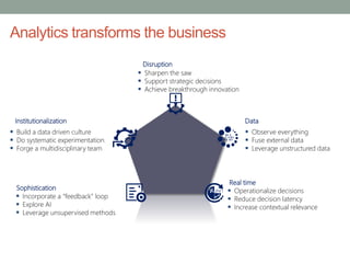
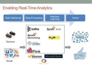
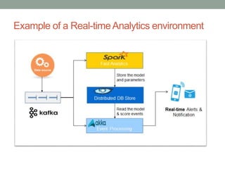
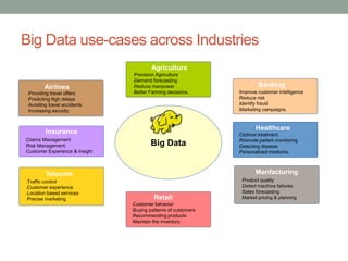
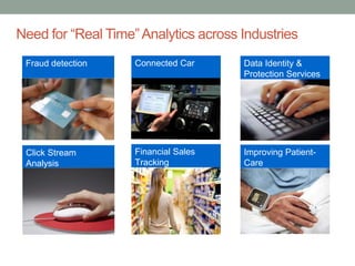
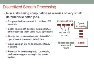
The document discusses real-time streaming analytics and its applications across various industries such as banking, healthcare, and retail, leveraging Apache Spark for processing large volumes of data efficiently. It details the capabilities of Spark Streaming for stateful stream processing, fault tolerance, and the integration of batch and streaming analytics. Additionally, it explores machine learning techniques, including clustering and online learning, emphasizing the importance of real-time data in driving business decisions and innovation.

1. REAL TIME STREAMING
ANALYTICS

2. About me
• Padma Chitturi
• Analytics Lead @ Fractal Analytics
• Author of “Apache Spark for
DataScience cookbook”
• https://github.com/ChitturiPadma/S
parkforDataScienceCookbook

3. Big Data use-cases across Industries
Banking
lImprove customer intelligence
lReduce risk
lIdentify fraud
lMarketing campaigns.
Healthcare
lOptimal treatment
lRremote patient monitoring
lDetecting disease
lPersonalized medicine.
Manfacturing
lProduct quality
lDetect machine failures
lSales forecasting
lMarket pricing & planningRetail
lCustomer behavior
lBuying patterns of customers
lRecommending products
lMaintain the inventory.
Telecom
lTraffic control
lCustomer experience
lLocation based services
lPrecise marketing
Insurance
lClaims Management
lRisk Management
lCustomer Experience & Insight
Airlines
lProviding travel offers
lPredicting fligh delays
lAvoiding travel accidents
lIncreasing security
Big Data
Agriculture
lPrecision Agriculture
lDemand forecasting
lReduce manpower
lBetter Farming decisions.

4. Need for “Real Time”Analytics across Industries
Fraud detection Connected Car Data Identity &
Protection Services
Click Stream
Analysis
Financial Sales
Tracking
Improving Patient-
Care

5. Overview of Spark
• In-memory cluster computing framework for processing
and analyzing large volumes of data.
• Key Features:
• Easy to use ( expressive API for batch & real-time processing
• Fast (provides in-memory persisting and optimizes disk seeks)
• General-purpose (support batch, real-time and graph processing).
• Scalable (as the data grows, computational power can be
increased by adding more nodes).
• Fault-tolerant (handles node failures without interrupting the
application by launching tasks on the nodes having replicated
copy)

6. What is Spark Streaming ?
• Extends Spark for doing large scale stream processing
• Scales to 100s of nodes and achieves second scale
latencies
• Efficient and fault-tolerant stateful stream processing
• Integrates with Spark’s batch and interactive processing
• Provides a simple batch-like API for implementing
complex algorithms.

7. Discretized Stream Processing
• Run a streaming computation as a series of very small,
deterministic batch jobs.
 Chop up the live stream into batches of X
seconds
 Spark treats each batch of data as RDDs
and processes them using RDD operations
 Finally, the processed results of the RDD
operations are returned in batches
 Batch sizes as low as ½ second, latency ~
1 second
 Potential for combining batch processing
and streaming processing in the same
system
Spark
Streaming
Spark
processed
results
Live data stream
batches of X
seconds

8. Example 1 – Get hashtags from Twitter
val tweets = ssc.twitterStream(<Twitter username>, <Twitter
password>)
Twitter Streaming API
batch @ t+1batch @ t batch @ t+2
tweets DStream
stored in memory as an RDD
(immutable, distributed dataset)

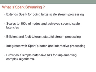
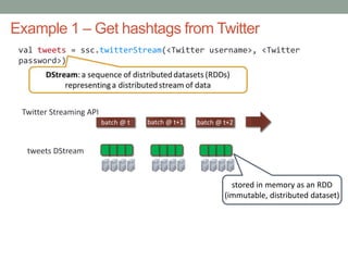
9. Example 1 – Get hashtags from Twitter
val tweets = ssc.twitterStream(<Twitter username>, <Twitter
password>)
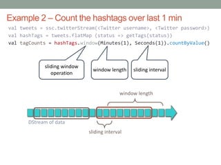
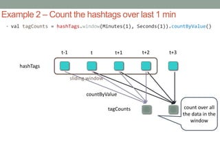
val hashTags = tweets.flatMap (status => getTags(status))
new DStream
transformation: modify data in one DStream to create
another DStream
batch @ t+1batch @ t batch @ t+2
flatMap flatMap flatMap
hashTags Dstream
[#cat, #dog, … ]
new RDDs created
for every batch
tweets Dstream

10. val tweets = ssc.twitterStream(<Twitter username>, <Twitter password>)
val hashTags = tweets.flatMap (status => getTags(status))
val tagCounts = hashTags.window(Minutes(1), Seconds(1)).countByValue()
Example 2 – Count the hashtags over last 1 min
sliding window
operation
window length sliding interval
DStream of data
window length
sliding interval

11. • val tagCounts = hashTags.window(Minutes(1), Seconds(1)).countByValue()
Example 2 – Count the hashtags over last 1 min
tagCounts
hashTags
t-1 t t+1 t+2 t+3
sliding window
countByValue
count over all
the data in the
window

12. Fault-tolerance
• RDDs remember the operations that
created them
• Batches of input data are replicated
in memory for fault-tolerance
• Data lost due to worker failure, can
be recomputed from replicated input
data
• Therefore, all transformed data is
fault-tolerant
input data
replicated
in memory
flatMap
lost partitions
recomputed on
other workers
tweets
RDD
hashTags
RDD

13. Fault-tolerance
• Spark Streaming program
t = ssc.twitterStream(“…”)
.map(…)
t.foreach(…)
t1 = ssc.twitterStream(“…”)
t2 = ssc.twitterStream(“…”)
t = t1.union(t2).map(…)
t.saveAsHadoopFiles(…)
t.map(…).foreach(…)
t.filter(…).foreach(…)
DStream Graph
T
M
F
E
Twitter Input DStream
Mapped DStream
Foreach DStreamDummy DStream signifying
an output operation
T
U
M
T
M FF
E
F
E
F
E

14. Dstream Graph -> RDD Graphs -> Spark Jobs
• Every interval, RDD graph is computed from DStream graph
• For each output operation, a Spark action is created
• For each action, a Spark job is created to compute it
T
U
M
T
M FF
E
F
E
F
E
DStream Graph RDD GraphBlock RDDs with
data received in
last batch interval B
U
M
B
M FA
A A
3 Spark Jobs

15. Execution Model – Job Scheduling
• Spark Streaming +Spark Driver
Network
Input
Tracker
Job
Scheduler Spark’s
Schedulers
DStream
Graph
Job
Manager
JobQueue
Jobs
Block IDsRDDs
Spark Workers
Jobs executed on
worker nodes
Block
Manager
Data
Received
Block
Manager

16. RDD Checkpointing
Saving RDD to HDFS to prevent RDD graph from growing too large
• Done internally in Spark transparent to the user program
• Done lazily, saved to HDFS the first time it is computed
red_rdd.checkpoint() HDFS file
Contents of red_rdd saved
to a HDFS file
transparent to
all child RDDs

17. RDD Checkpointing
Stateful DStream operators can have infinite lineages
data
t-1 t t+1 t+2 t+3
states
Large lineages lead to …
• Large closure of the RDD object  large task sizes  high task launch
times
• High recovery times under failure
• Periodic RDD Check-pointing solves this
• Useful for iterative Spark programs as well.
HDF
S
HDF
S

18. Performance Tuning
• Increase Read parallelism
• Increase downstream processing parallelism
• Achieve stable configuration that can sustain the
streaming workload
• Optimize for low-latency
• Memory settings and explore GC options.
• Achieve Fault-tolerance
• Serializing the objects.

19. Analytics transforms the business
Institutionalization
Real time
Data
Sophistication
 Sharpen the saw
 Support strategic decisions
 Achieve breakthrough innovation
 Observe everything
 Fuse external data
 Leverage unstructured data
 Incorporate a “feedback” loop
 Explore AI
 Leverage unsupervised methods
 Build a data driven culture
 Do systematic experimentation
 Forge a multidisciplinary team
 Operationalize decisions
 Reduce decision latency
 Increase contextual relevance
Disruption

20. Enabling Real-TimeAnalytics
Sensors
Social

21. Machine Learning
• It is derived from the concept that it deals with “construction
and study of systems that can learn from data”
• It is seen as building blocks to make computers learn to
behave more intelligently.
• Two phases in learning process – training & testing
• Two kinds of learning
• Unsupervised
• no labels in the training data
• Algorithms detects the patterns in the data and groups the
observations of similar characteristics together
• Supervised
• We have training data with correct labels
• Use training data to prepare the algorithm
• Then apply it to data without a correct label

22. Some types of algorithms
• Prediction
• predicting variable from data
• Classification
• Assigning observations to pre-defined classes
• Clustering
• Splitting observations into groups based on similarity
• Recommendation
• Predicts what people might like & uncovers relationship between
items.

23. Steps in Analytics Workload
• Data Collection
• Pre-processing the data (cleaning & data munging)
• Retrieve sample data from the actual population
• Descriptive statistics on the sample data
• Exploratory Data Analysis with Spark
• Uni-variate analysis
• Bivariate analysis
• Missing Value treatment
• Outlier- detection
• Feature Engineering
• Apply machine learning models
• Optimize and fine-tune the model parameters

24. Sample Data
Types of labels:
• Denial of service (DoS – attack type)
• Normal
• Probe (attack)
• R2L (attack)
• U2R(attack)

25. Unsupervised Learning - Clustering
• Clustering is the assignment of a set of observations into subsets
(called clusters) so that observations in the same cluster are similar in
some sense.
• Find areas dense with data (also area without
• data)
• Anomaly – far from any cluster
• Supervise with labels to improve,
interpret

26. Streaming K-means (K-means ++)
• Assign points to nearest center, update centers, iterate
• Goal: points close to nearest cluster center
• Must choose k = number of clusters
• ++ means smarter starting point

27. Clustering – choosing parameters
• Initial plotted tsne plot which gives the
distribution of data in 2 dimensions. It helps
to identify if the data can be clustered.
• Normalize the data before applying k-means
i.e. standardize the scores as
• Choose k value using elbow method or
using PCA analysis
• Convert categorical variables to numeric
using one-hot encoding
tsne plot
elbow plot

28. Streaming k-means
Approach:
Start with k cluster centres initially
For every incoming batch of data, centroids keep updating.
The clusters drift over time, and after certain stage, they stabilize.
Continuously learns new data patterns.
Outliers are detected as anomalies.
Pros:
More useful when the data points don't have labels associated with them.
Simple to implement.
Cons:
Doesn't fit for high dimension data.
Kafka
Streaming
K-means
Network
Data

29. “Offline” vs “Online” algorithms
 Build models on static data
 Train algorithms on “batches” of data
 Use the model to make predictions on
incoming data stream
• Pros:
 Easy to analyze
 High accuracy
 Batch algorithms are quite accessible.
• Cons:
 Unable to identify dynamic patterns
 Build model on live stream of data
 Training happens continuously on live
data
 Use the model for both predict and learn
on streaming data.
• Pros:
 Model evolves continuously.
 Identifies rapidly changing patterns in
the data.
• Cons:
 Streaming algorithms are not widely
available.
 Active area of research
Offline Learning Online Learning

30. Streaming SVM
In machine learning, support vector machines (SVM) are supervised learning
models with associated learning algorithms that analyze data used for classification
and regression analysis.
 Capable of reflecting changes of dataset real time.
SVM is resistive to noise.
It uses high dimension to separate dataset.
Prediction rate can be increased by scaling the Spark cluster.

31. Example of a Real-timeAnalytics environment