Downloaded 14 times

![Fundamentals (contd.)
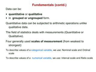
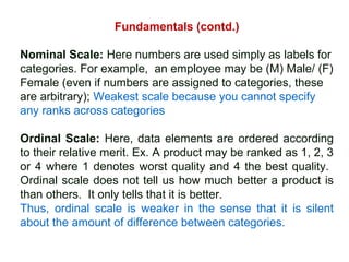
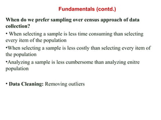
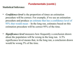
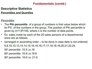
• Ratio Scale: An ordered scale in which the difference between
measurement is an meaningful quantity and involves a true 0 point (0
is in ratio scale is an absolute 0). Strongest scale.
• If two measurements are in ratio scale, then we can take ratios of
those measurements.
Ex. Money is measured in ratio scale. A sum of Rs. 0 means no
money and is thus an absolute zero. A sum of Rs. 100 is twice as
large as Rs. 50. Other examples are height, weight, volume, area,
length.
[Note that in interval scale, the interval between two interval scale
measurements is in ratio scale (not the individual observations). ]](https://image.slidesharecdn.com/qt-businessstatistics-lesson1-2013-130830214815-phpapp02/85/Qt-business-statistics-lesson1-2013-7-320.jpg)

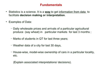
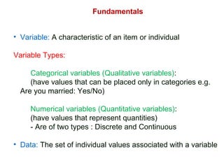
This document provides an overview of fundamental statistical concepts. It defines statistics as a science used to obtain information from data to facilitate decision making. It discusses different types of variables and scales of measurement used in statistics. It also describes key concepts such as population and sample, different sampling methods, descriptive statistics including measures of central tendency, and how statistical inference is used to generalize from samples to populations. Examples are provided to illustrate concepts throughout.


![Getting Started with Apache Spark: Big Data Made Simple [Free Meetup]](https://cdn.slidesharecdn.com/ss_thumbnails/apachesparkgettingstarted-260203175547-8361bcc3-thumbnail.jpg?width=640&height=640&fit=bounds)


