DATA preprocessing.pptx

1
Module 3: Data Pre-processing

So far : Research Problem
2
NIT Delhi
Source : https://developers.google.com/machine-learning/crash-course

Data Collection and Creation
• Using Already Available data:
– Google Dataset : [ https://datasetsearch.research.google.com/ ]
– Kaggle : [ https://www.kaggle.com/ ]
– UCI Machine Learning Repository : [https://archive.ics.uci.edu/ml/index.php ]
– Paper with code: [ https://paperswithcode.com/ ]
– NLP-progress : [http://nlpprogress.com/]
– Open Government Data (OGD) Platform India [ https://data.gov.in/]
• Other Papers: [https://scholar.google.com/]
• Google Patents : [https://patents.google.com/]
– Why to choose
– Effort of Creating and filtering reduces
– Base Line
– Explore new Computational techniques
– Life easy
3
NIT Delhi

Module 3 : Data Pre-processing
• Data Preprocessing: An Overview
– Data Quality
– Major Tasks in Data Preprocessing
• Data Cleaning
• Data Integration
• Data Reduction
• Data Transformation and Data Discretization
5
NIT Delhi

Transform data in ML Problem
Preprocessing
Feature
Extraction
Raw
data
Processed
data
Feature
Vectors
source: Practical Machine Learning with Python, Apress/Springer

Need of Pre-Processing
7
NIT Delhi

A Machine Learning System
Preprocessing
Feature
Extraction
Machine
Learner
Classifier
Output
Raw
Data
Formatted
Data
Testing
Examples
Function
Parameters
Labels
Feature
Vectors
Training
Examples

Need for Feature Engineering
Source: https://www.forbes.com/sites/gilpress/2016/03/23/data-preparation-most-time-consuming-least-enjoyable-data-science-task-survey-
says/ 10
NIT Delhi
“Coming up with features is difficult, time-consuming, requires expert knowledge.
‘Applied machine learning’is basically feature engineering.”
— Prof. Andrew Ng.

Feature Engineering
• Data Types:
– Structured data - Tabular data
– Semi-structured data - Json data
– Unstructured data - Text file
12
NIT Delhi
1.Data
reading
Data Pre-
processing
Data
Visualization
Dimension
Reduction
1.Feature
Selection
1.Feature
Extraction
Exploratory Data Analysis ( EDA )

Module 3: Data Preprocessing
– Data Quality
• Data Cleaning
• Data Reduction
• Summary
13
13

Data Quality: Why Preprocess the Data?
• Measures for data quality: A multidimensional view
– Accuracy: correct or wrong, accurate or not
– Completeness: not recorded, unavailable, …
– Consistency: some modified but some not, dangling, …
– Timeliness: timely update?
– Believability: how trustable the data are correct?
– Interpretability: how easily the data can be understood?
14

Major Tasks in Data Preprocessing
• Data cleaning
– Fill in missing values, smooth noisy data, identify or remove outliers, and resolve inconsistencies
• Data integration
– Integration of multiple databases, data cubes, or files
• Data reduction
– Dimensionality reduction
– Numerosity reduction
– Data compression
• Data transformation and data discretization
– Normalization
– Concept hierarchy generation
15

Module 3: Data Preprocessing
– Data Quality
• Data Cleaning
• Data Reduction
• Summary
16
16

Data Cleaning
• Data in the Real World Is Dirty: Lots of potentially incorrect data, e.g., instrument faulty, human or
computer error, transmission error
– incomplete: lacking attribute values, lacking certain attributes of interest, or containing only
aggregate data
• e.g., Occupation=“ ” (missing data)
– noisy: containing noise, errors, or outliers
• e.g., Salary=“−10” (an error)
– inconsistent: containing discrepancies in codes or names, e.g.,
• Age=“42”, Birthday=“03/07/2010”
• Was rating “1, 2, 3”, now rating “A, B, C”
• discrepancy between duplicate records
– Intentional (e.g., disguised missing data)
• Jan. 1 as everyone’s birthday?
17

Incomplete (Missing) Data
• Data is not always available
– E.g., many tuples have no recorded value for several attributes, such as
customer income in sales data
• Missing data may be due to
– equipment malfunction
– inconsistent with other recorded data and thus deleted
– data not entered due to misunderstanding
– certain data may not be considered important at the time of entry
– not register history or changes of the data
• Missing data may need to be inferred
18

How to Handle Missing Data?
• Ignore the tuple: usually done when class label is missing (when doing classification)
– not effective when the % of missing values per attribute varies considerably
• Fill in the missing value manually: tedious + infeasible?
• Fill in it automatically with
– a global constant : e.g., “unknown”, a new class?!
– the attribute mean
– the attribute mean for all samples belonging to the same class: smarter
– the most probable value: inference-based such as Bayesian formula or decision
tree
19

20
Noisy Data
• Noise: random error or variance in a measured variable
• Incorrect attribute values may be due to
– faulty data collection instruments
– data entry problems
– data transmission problems
– technology limitation
– inconsistency in naming convention
• Other data problems which require data cleaning
– duplicate records
– incomplete data
– inconsistent data

How to Handle Noisy Data?
• Binning
– first sort data and partition into (equal-frequency) bins
– then one can smooth by bin means, smooth by bin median, smooth by bin
boundaries, etc.
• Regression
– smooth by fitting the data into regression functions
• Clustering
– detect and remove outliers
• Combined computer and human inspection
– detect suspicious values and check by human (e.g., deal with possible outliers)
21

Data Cleaning as a Process
• Data discrepancy detection
– Use metadata (e.g., domain, range, dependency, distribution)
– Check field overloading
– Check uniqueness rule, consecutive rule and null rule
– Use commercial tools
• Data scrubbing: use simple domain knowledge (e.g., postal code, spell-check) to detect errors and
make corrections
• Data auditing: by analyzing data to discover rules and relationship to detect violators (e.g.,
correlation and clustering to find outliers)
• Data migration and integration
– Data migration tools: allow transformations to be specified
– ETL (Extraction/Transformation/Loading) tools: allow users to specify transformations through a
graphical user interface
• Integration of the two processes
– Iterative and interactive (e.g., Potter’s Wheels)
22

1. Pre-processing : Tabular data
• Data reading
• Missing Values
– The reason for the missing values might be human errors, interruptions in the data
flow, privacy concerns, and so on
– Drop the rows or the entire column. (70%)
– Numerical Imputation
• Replace missing value
– Categorical Imputation
• Fill missing with mean
• Handling Outliers
– Demonstrate the data visually
– Statistical methodologies:
• Standard deviation, and
• Percentiles : (Assume a certain percent of the value from the top or the bottom as an outlier)
– An Outlier Dilemma: Drop or Cap
23
NIT Delhi

Features Encoding and Decoding
• Need to encode each input data as a vector in Rn:
• Label Encoding
– One-hot encoding
• How to treat “real” learning problems in this framework?
24
600.325/425 Declarative Methods - J. Eisner

Type of encoding
Output Encoding types:-
• Local Encoding
– Different output values represent different classes,
– e.g.
• <0.2 – class 1,
• >0.8 – class 2,
• in between – ambiguous class (class 3)
• Distributed (binary, 1-of-n) Encoding
– is typically used in multi class problems
– Number of outputs = number of classes
– Example: 3 classes, 3 output neurons;
• class 1 - as 1 0 0
• class 2 - as 0 1 0
• class 3 - as 0 0 1
25
NIT Delhi

Pre-processing : Tabular data
• Log Transform
– handle skewed data and after transformation, the distribution becomes more approximate to normal.
– decreases the effect of the outliers
• Binning
– Binning can be applied on both categorical and numerical data
– model more robust and prevent overfitting
• Scaling/ Normalization
– Need of Normalization
– Type of Normalization
– Min-Max Normalization:
– Standard Normalization / Standardization : Z-score Normalization:
– Where μ is mean and σ is standard deviation
– Mean or Normal Mean
• Feature Split / Joining
26
NIT Delhi

2. Data Visualization
27
NIT Delhi
https://xkcd.com/1838/

Inspect the data
• Spend a lot of time looking at data
• Spend some more time with data (in hours )
• Look at data biases, errors
• Try to observe how your brain classifies the data. This would tell you:-
– What type of pre processing to be used
– What type of model you should use
– Will give you human baseline
• Build graph, look for distributions, errors and correlation in data
28
NIT Delhi

Nonlinear Separators
x
y
Note: A more complex function
requires more data to generate
an accurate model
(sample complexity)

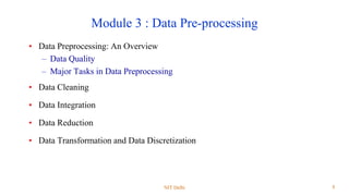
Pre-processing : Tabular data
• Class Imbalance –
– Synthetic Minority Over-sampling Technique ( SMOTE )
• Example in python
– [Tabular_data.ipynb]
31
NIT Delhi

Image Processing using CV2 and PIL
• Load and read image
• Convert color image into grayscale
• Resize image
• Rotate image
• Scaling
• Edge Detection
• Applying Noise Removing
• Image Segmentation.
• Morphology
32
NIT Delhi

Features
• Features: Information from the raw data that is most relevant for discrimination between the
classes
– Extract features with low within-class variability and high between class variability
– Discard redundant information
• A feature is typically a specific representation on top of raw data
– Feature Engineering on Numeric Data
– Statistical Transformations
34
NIT Delhi

Features for recognizing a chair?
35

Features for recognizing a chair?
• Feature Extraction
• Binary Object Features (Area, Center of Area, Axis of Least Second Moment, Perimeter,
Thinness Ratio, Irregularity, Aspect Ratio, Euler Number, Projection)
• Histogram Features (Mean, Standard Deviation, Skew, Energy, Entropy)
• Color Features
• Spectral Features
• Feature Analysis
• Feature Vectors and Feature Spaces
– Distance and Similarity Measures (Euclidean distance, Range-normalized Euclidean
distance, City block or absolute value metric, Maximum value)

Feature Analysis
• Feature analysis argues that we observe individual characteristics,
or features, of every object and pattern we encounter.
– Relation among the variablesfeatures
– Data Visualization
Too many features
1. Feature Reduction
2. Feature Selection
3. Feature Extraction
37
NIT Delhi

Embedding
• Requires some knowledge engineering
• Makes the discriminant function simpler (and learnable)
X2
X1
5
2
3
3
4
1
3
2
1 x
x
x
x
x
x
x
x
x 

5
4
1 y
y
y 


Feature Analysis
• Feature contain information about target
• How to choose a good set of features?
– Discriminative features
– Invariant features (e.g., translation, rotation and scale)
• Are there ways to automatically learn which features are best ?
• Extract the information from the raw data that is most relevant for discrimination between the
classes
• Extract features with low within-class variability and high between class variability
• Discard redundant information
39

Feature
- The information about the target class is inherent in the variables.
- Naïve view:
More features
=> More information
=> More discrimination power.
- In practice:
many reasons why this is not the case!

How Many Features?
• Does adding more features always improve performance?
• No
– Irrelevant features (introduce noise)
– Redundant features – no additional information
– It might be difficult and computationally expensive to extract certain features.
– Correlated features might not improve performance.
– “Curse” of dimensionality occurs: -
• When no of training example is fixed and
• limited computational resources
41

Curse of Dimensionality
• Adding too many features can, paradoxically, lead to a worsening of
performance.
– Divide each of the input features into a number of intervals, so that the value of a feature can
be specified approximately by saying in which interval it lies.
– If each input feature is divided into M divisions, then the total number of cells is Md (d: # of
features).
– Since each cell must contain at least one point, the number of training data grows
exponentially with d.
42

• Number of training examples is fixed
– the classifier’s performance usually will degrade for a large number of
features!

44

When no of training example is fixed and

Limited computational resources

Feature Reduction in ML
- Irrelevant and
- Redundant features
- can confuse learners.
- Limited training data.
- Limited computational resources.
- Curse of dimensionality.

Why Dimensionality Reduction?
- Irrelevant and Redundant features
- can confuse learners.
• It is so easy and convenient to collect data
– an experiment
• Dimensionality reduction is an effective approach to downsizing data
• Most machine learning and data mining techniques may not be effective for
high-dimensional data
– Curse of Dimensionality
– Query accuracy and efficiency degrade rapidly as the dimension
increases.
46

Why Dimensionality Reduction?
• The intrinsic dimension may be small.
– For example, the number of genes responsible for a certain
type of disease may be small.
• Visualization: projection of high-dimensional data onto 2D or
3D.
• Data compression: efficient storage and retrieval.
• Noise removal: positive effect on query accuracy.
47

Document Classification
48
Internet
ACM Portal PubMed
IEEE Xplore
Digital Libraries
Web Pages
Emails
 Task: To classify unlabeled
documents into categories
 Challenge: thousands of terms
 Solution: to apply dimensionality
reduction
D1
D2
Sports
T1 T2 ….…… TN
12 0 ….…… 6
DM
C
Travel
Jobs
…
…
…
Terms
Documents
3 10 ….…… 28
0 11 ….…… 16
…

Module3: Data Preprocessing
– Data Quality
• Data Cleaning
• Data Reduction
• Summary
49
49

Data Integration
• Data integration:
– Combines data from multiple sources into a coherent store
• Schema integration: e.g., A.cust-id  B.cust-#
– Integrate metadata from different sources
• Entity identification problem:
– Identify real world entities from multiple data sources, e.g., Bill Clinton = William Clinton
• Detecting and resolving data value conflicts
– For the same real world entity, attribute values from different sources are different
– Possible reasons: different representations, different scales, e.g., metric vs. British units
50
50

Handling Redundancy in Data Integration
• Redundant data occur often when integration of multiple databases
– Object identification: The same attribute or object may have different names in
different databases
– Derivable data: One attribute may be a “derived” attribute in another table, e.g.,
annual revenue
• Redundant attributes may be able to be detected by correlation analysis and
covariance analysis
• Careful integration of the data from multiple sources may help reduce/avoid
redundancies and inconsistencies and improve mining speed and quality
51
51

Correlation Analysis (Nominal Data)
• Χ2 (chi-square) test
• The larger the Χ2 value, the more likely the variables are related
• The cells that contribute the most to the Χ2 value are those whose actual count is
very different from the expected count
• Correlation does not imply causality
– # of hospitals and # of car-theft in a city are correlated
– Both are causally linked to the third variable: population



Expected
Expected
Observed 2
2 )
(

52

Chi-Square Calculation: An Example
• Χ2 (chi-square) calculation (numbers in parenthesis are expected counts
calculated based on the data distribution in the two categories)
• It shows that like_science_fiction and play_chess are correlated in the group
93
.
507
840
)
840
1000
(
360
)
360
200
(
210
)
210
50
(
90
)
90
250
( 2
2
2
2
2










53
Play chess Not play chess Sum (row)
Like science fiction 250(90) 200(360) 450
Not like science fiction 50(210) 1000(840) 1050
Sum(col.) 300 1200 1500

Correlation Analysis (Numeric Data)
• Correlation coefficient (also called Pearson’s product moment coefficient)
where n is the number of tuples, and are the respective means of A and B,
σA and σB are the respective standard deviation of A and B, and
Σ(aibi) is the sum of the AB cross-product.
• If rA,B > 0, A and B are positively correlated (A’s values increase as B’s).
– The higher, the stronger correlation.
• rA,B = 0: independent; rAB < 0: negatively correlated
B
A
n
i i
i
B
A
n
i i
i
B
A
n
B
A
n
b
a
n
B
b
A
a
r



 )
1
(
)
(
)
1
(
)
)(
( 1
1
,








 

A
54
B

Visually Evaluating Correlation
55
Scatter plots showing the
similarity from –1 to 1.

Correlation (viewed as linear relationship)
• Correlation measures the linear relationship between objects
• To compute correlation,
– we standardize data objects, A and B, and then take their dot product
56
)
(
/
))
(
(
' A
std
A
mean
a
a k
k 

)
(
/
))
(
(
' B
std
B
mean
b
b k
k 

'
'
)
,
( B
A
B
A
n
correlatio 


Covariance (Numeric Data)
• Covariance is similar to correlation
where n is the number of tuples, and are the respective mean or expected values of A
and B, σA and σB are the respective standard deviation of A and B.
• Positive covariance: If CovA,B > 0, then A and B both tend to be larger than their expected
values.
• Negative covariance: If CovA,B < 0 then if A is larger than its expected value, B is likely to be
smaller than its expected value.
• Independence: CovA,B = 0 but the converse is not true:
– Some pairs of random variables may have a covariance of 0 but are not independent. Only under
some additional assumptions (e.g., the data follow multivariate normal distributions) does a
covariance of 0 imply independence 57
A B
Correlation coefficient:

Co-Variance: An Example
• It can be simplified in computation as
• Suppose two stocks A and B have the following values in one week: (2, 5), (3, 8), (5, 10), (4,
11), (6, 14).
• Question: If the stocks are affected by the same industry trends, will their prices rise or fall
together?
– E(A) = (2 + 3 + 5 + 4 + 6)/ 5 = 20/5 = 4
– E(B) = (5 + 8 + 10 + 11 + 14) /5 = 48/5 = 9.6
– Cov(A,B) = (2×5+3×8+5×10+4×11+6×14)/5 − 4 × 9.6 = 4
• Thus, A and B rise together since Cov(A, B) > 0.

Forms of data pre-processing
59

60
– Data Quality
• Data Cleaning
• Data Reduction
• Summary
60

Data Reduction Strategies
• Data reduction: Obtain a reduced representation of the data set that is much smaller in volume but
yet produces the same (or almost the same) analytical results
• Why data reduction? — A database/data warehouse may store terabytes of data. Complex data
analysis may take a very long time to run on the complete data set.
• Data reduction strategies
– Dimensionality reduction, e.g., remove unimportant attributes
• Wavelet transforms
• Principal Components Analysis (PCA)
• Feature subset selection, feature creation
– Numerosity reduction (some simply call it: Data Reduction)
• Regression and Log-Linear Models
• Histograms, clustering, sampling
• Data cube aggregation
61

62
Data Reduction 1: Dimensionality Reduction
• Curse of dimensionality
– When dimensionality increases, data becomes increasingly sparse
– Density and distance between points, which is critical to clustering, outlier
analysis, becomes less meaningful
– The possible combinations of subspaces will grow exponentially
• Dimensionality reduction
– Avoid the curse of dimensionality
– Help eliminate irrelevant features and reduce noise
– Reduce time and space required in data mining
– Allow easier visualization
• Dimensionality reduction techniques
– Wavelet transforms
– Principal Component Analysis
– Supervised and nonlinear techniques (e.g., feature selection)

63
Mapping Data to a New Space
Two Sine Waves Two Sine Waves + Noise Frequency
 Fourier transform
 Wavelet transform

64
What Is Wavelet Transform?
• Decomposes a signal into
different frequency subbands
– Applicable to n-dimensional
signals
• Data are transformed to preserve
relative distance between objects
at different levels of resolution
• Allow natural clusters to become
more distinguishable
• Used for image compression

65
Wavelet Transformation
• Discrete wavelet transform (DWT) for linear signal processing, multi-resolution
analysis
• Compressed approximation: store only a small fraction of the strongest of the
wavelet coefficients
• Similar to discrete Fourier transform (DFT), but better lossy compression,
localized in space
• Method:
– Length, L, must be an integer power of 2 (padding with 0’s, when necessary)
– Each transform has 2 functions: smoothing, difference
– Applies to pairs of data, resulting in two set of data of length L/2
– Applies two functions recursively, until reaches the desired length
Haar2 Daubechie4

67
Haar Wavelet Coefficients
Coefficient “Supports”
2 2 0 2 3 5 4 4
-1.25
2.75
0.5 0
0 -1 0
-1
+
-
+
+
+ + +
+
+
- -
- - - -
+
-
+
+ -
+ -
+-
+-
-
+
+-
-1
-1
0.5
0
2.75
-1.25
0
0
Original frequency distribution
Hierarchical
decomposition
structure (a.k.a.
“error tree”)

68
Why Wavelet Transform?
• Use hat-shape filters
– Emphasize region where points cluster
– Suppress weaker information in their boundaries
• Effective removal of outliers
– Insensitive to noise, insensitive to input order
• Multi-resolution
– Detect arbitrary shaped clusters at different scales
• Efficient
– Complexity O(N)
• Only applicable to low dimensional data

Principal Component Analysis (PCA)
• Find a projection that captures the largest amount of variation in data
• The original data are projected onto a much smaller space, resulting in dimensionality
reduction. We find the eigenvectors of the covariance matrix, and these eigenvectors define
the new space
69
x2
x1
e

Principal Component Analysis
• Principal component analysis (PCA)
– Reduce the dimensionality of a data set by finding a new set of
variables, smaller than the original set of variables
– Retains most of the sample's information.
• By information we mean the variation present in the
sample, given by the correlations between the original
variables.
– The new variables, called principal components (PCs), are
uncorrelated, and are ordered by the fraction of the total
information each retains.
70

Principal Component Analysis (Steps)
• Given N data vectors from n-dimensions, find k ≤ n orthogonal vectors (principal components)
that can be best used to represent data
– Normalize input data: Each attribute falls within the same range
– Compute k orthonormal (unit) vectors, i.e., principal components
– Each input data (vector) is a linear combination of the k principal component vectors
– The principal components are sorted in order of decreasing “significance” or strength
– Since the components are sorted, the size of the data can be reduced by eliminating the
weak components, i.e., those with low variance (i.e., using the strongest principal
components, it is possible to reconstruct a good approximation of the original data)
• Works for numeric data only
71

PCA
• Assume that N features are linear combination of M < 𝑁 vectors
𝑧𝑖 = 𝑤𝑖1𝑥𝑖1 + ⋯ + 𝑤𝑖𝑑𝑥𝑖𝑁
• What we expect from such basis
– Uncorrelated or otherwise can be reduced further
– Have large variance (e.g. 𝑤𝑖1 have large variation) or otherwise bear no
information

Geometric picture of principal components (PCs)

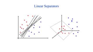
Algebraic definition of PCs
.
,
,
2
,
1
,
1
1
1
1 p
j
x
a
x
a
z
N
i
ij
i
j
T



 

  N
p
x
x
x 

,
,
, 2
1 
]
var[ 1
z
)
,
,
,
(
)
,
,
,
(
2
1
1
21
11
1
Nj
j
j
j
N
x
x
x
x
a
a
a
a




Given a sample of p observations on a vector of N variables
define the first principal component of the sample
by the linear transformation
where the vector
is chosen such that is maximum.

• Choose directions such that a total variance of data will be maximum
– Maximize Total Variance
• Choose directions that are orthogonal
– Minimize correlation
• Choose 𝑀 < 𝑁 orthogonal directions which maximize total variance

PCA
• 𝑁-dimensional feature space
• N × 𝑁 symmetric covariance matrix estimated from samples 𝐶𝑜𝑣 𝒙
= Σ
• Select 𝑀 largest eigenvalue of the covariance matrix and associated
𝑀 eigenvectors
• The first eigenvector will be a direction with largest variance

PCA for image compression
p=1 p=2 p=4 p=8
p=16 p=32 p=64 p=100
Original
Image

Is PCA a good criterion for classification?
• Data variation
determines the
projection direction
• What’s missing?
– Class information

What is a good projection?
• Similarly, what is a good
criterion?
– Separating different classes
Two classes
overlap
Two classes are
separated

What class information may be useful?
Within-class distance
• Between-class distance
– Distance between the centroids of
different classes
• Within-class distance
• Accumulated distance of an instance to
the centroid of its class
• Linear discriminant analysis (LDA) finds
most discriminant projection by
• maximizing between-class distance
• and minimizing within-class distance

Linear Discriminant Analysis
• Find a low-dimensional space such that when 𝒙 is
projected, classes are well-separated

Good Projection
• Means are as far away as possible
• Scatter is small as possible
• Fisher Linear Discriminant
 
 
2
1 2
2 2
1 2
m m
J
s s



w

Attribute Subset Selection
• Another way to reduce dimensionality of data
• Redundant attributes
– Duplicate much or all of the information contained in one or more other
attributes
– E.g., purchase price of a product and the amount of sales tax paid
• Irrelevant attributes
– Contain no information that is useful for the data mining task at hand
– E.g., students' ID is often irrelevant to the task of predicting students' GPA
86

Heuristic Search in Attribute Selection
• There are 2d possible attribute combinations of d attributes
• Typical heuristic attribute selection methods:
– Best single attribute under the attribute independence assumption: choose
by significance tests
– Best step-wise feature selection:
• The best single-attribute is picked first
• Then next best attribute condition to the first, ...
– Step-wise attribute elimination:
• Repeatedly eliminate the worst attribute
– Best combined attribute selection and elimination
– Optimal branch and bound:
• Use attribute elimination and backtracking
87

88
Attribute Creation (Feature Generation)
• Create new attributes (features) that can capture the important information in a
data set more effectively than the original ones
• Three general methodologies
– Attribute extraction
• Domain-specific
– Mapping data to new space (see: data reduction)
• E.g., Fourier transformation, wavelet transformation, manifold
approaches (not covered)
– Attribute construction
• Combining features (see: discriminative frequent patterns in Module7)
• Data discretization

Data Reduction 2: Numerosity Reduction
• Reduce data volume by choosing alternative, smaller forms of data representation
• Parametric methods (e.g., regression)
– Assume the data fits some model, estimate model parameters, store only the
parameters, and discard the data (except possible outliers)
– Ex.: Log-linear models—obtain value at a point in m-D space as the product
on appropriate marginal subspaces
• Non-parametric methods
– Do not assume models
– Major families: histograms, clustering, sampling, …
89

Parametric Data Reduction: Regression and
Log-Linear Models
• Linear regression
– Data modeled to fit a straight line
– Often uses the least-square method to fit the line
• Multiple regression
– Allows a response variable Y to be modeled as a linear function of
multidimensional feature vector
• Log-linear model
– Approximates discrete multidimensional probability distributions
90

Regression Analysis
• Regression analysis: A collective name for techniques
for the modeling and analysis of numerical data
consisting of values of a dependent variable (also
called response variable or measurement) and of one or
more independent variables (aka. explanatory variables
or predictors)
• The parameters are estimated so as to give a "best fit"
of the data
• Most commonly the best fit is evaluated by using the
least squares method, but other criteria have also been
used
• Used for prediction (including
forecasting of time-series data),
inference, hypothesis testing,
and modeling of causal
relationships
91
y
x
y = x + 1
X1
Y1
Y1’

Regress Analysis and Log-Linear Models
• Linear regression: Y = w X + b
– Two regression coefficients, w and b, specify the line and are to be estimated by using the data
at hand
– Using the least squares criterion to the known values of Y1, Y2, …, X1, X2, ….
• Multiple regression: Y = b0 + b1 X1 + b2 X2
– Many nonlinear functions can be transformed into the above
• Log-linear models:
– Approximate discrete multidimensional probability distributions
– Estimate the probability of each point (tuple) in a multi-dimensional space for a set of
discretized attributes, based on a smaller subset of dimensional combinations
– Useful for dimensionality reduction and data smoothing
92

Histogram Analysis
• Divide data into buckets and store
average (sum) for each bucket
• Partitioning rules:
– Equal-width: equal bucket range
– Equal-frequency (or equal-depth)
93
0
5
10
15
20
25
30
35
40
10000 30000 50000 70000 90000

Clustering
• Partition data set into clusters based on similarity, and store cluster representation
(e.g., centroid and diameter) only
• Can be very effective if data is clustered but not if data is “smeared”
• Can have hierarchical clustering and be stored in multi-dimensional index tree
structures
• There are many choices of clustering definitions and clustering algorithms
• Cluster analysis will be studied in depth in Module10
94

Sampling
• Sampling: obtaining a small sample s to represent the whole data set N
• Allow a mining algorithm to run in complexity that is potentially sub-linear to
the size of the data
• Key principle: Choose a representative subset of the data
– Simple random sampling may have very poor performance in the presence of
skew
– Develop adaptive sampling methods, e.g., stratified sampling:
• Note: Sampling may not reduce database I/Os (page at a time)
95

Types of Sampling
• Simple random sampling
– There is an equal probability of selecting any particular item
• Sampling without replacement
– Once an object is selected, it is removed from the population
• Sampling with replacement
– A selected object is not removed from the population
• Stratified sampling:
– Partition the data set, and draw samples from each partition
(proportionally, i.e., approximately the same percentage of the data)
– Used in conjunction with skewed data
96

97
Sampling: With or without Replacement
Raw Data

Sampling: Cluster or Stratified Sampling
98
Raw Data Cluster/Stratified Sample

100
Data Reduction 3: Data Compression
• String compression
– There are extensive theories and well-tuned algorithms
– Typically lossless, but only limited manipulation is possible without expansion
• Audio/video compression
– Typically lossy compression, with progressive refinement
– Sometimes small fragments of signal can be reconstructed without reconstructing
the whole
• Time sequence is not audio
– Typically short and vary slowly with time
• Dimensionality and numerosity reduction may also be considered as forms of data
compression

101
Data Compression
Original Data Compressed
Data
lossless
Original Data
Approximated

102
– Data Quality
• Data Cleaning
• Data Reduction
• Summary

103
Data Transformation
• A function that maps the entire set of values of a given attribute to a new set of replacement values s.t.
each old value can be identified with one of the new values
• Methods
– Smoothing: Remove noise from data
– Attribute/feature construction
• New attributes constructed from the given ones
– Aggregation: Summarization, data cube construction
– Normalization: Scaled to fall within a smaller, specified range
• min-max normalization
• z-score normalization
• normalization by decimal scaling
– Discretization: Concept hierarchy climbing

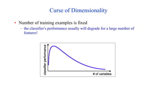
Normalization
• Min-max normalization: to [new_minA, new_maxA]
– Ex. Let income range $12,000 to $98,000 normalized to [0.0, 1.0].
Then $73,000 is mapped to
• Z-score normalization (μ: mean, σ: standard deviation):
– Ex. Let μ = 54,000, σ = 16,000. Then
• Normalization by decimal scaling
716
.
0
0
)
0
0
.
1
(
000
,
12
000
,
98
000
,
12
600
,
73





225
.
1
000
,
16
000
,
54
600
,
73


104
A
A
A
A
A
A
min
new
min
new
max
new
min
max
min
v
v _
)
_
_
(
' 




A
A
v
v




'
j
v
v
10
' Where j is the smallest integer such that Max(|ν’|) < 1

Discretization
• Three types of attributes
– Nominal—values from an unordered set, e.g., color, profession
– Ordinal—values from an ordered set, e.g., military or academic rank
– Numeric—real numbers, e.g., integer or real numbers
• Discretization: Divide the range of a continuous attribute into intervals
– Interval labels can then be used to replace actual data values
– Reduce data size by discretization
– Supervised vs. unsupervised
– Split (top-down) vs. merge (bottom-up)
– Discretization can be performed recursively on an attribute
– Prepare for further analysis, e.g., classification
105

106
Data Discretization Methods
• Typical methods: All the methods can be applied recursively
– Binning
• Top-down split, unsupervised
– Histogram analysis
• Top-down split, unsupervised
– Clustering analysis (unsupervised, top-down split or bottom-up merge)
– Decision-tree analysis (supervised, top-down split)
– Correlation (e.g., 2) analysis (unsupervised, bottom-up merge)

Simple Discretization: Binning
• Equal-width (distance) partitioning
– Divides the range into N intervals of equal size: uniform grid
– if A and B are the lowest and highest values of the attribute, the width of intervals will be:
W = (B –A)/N.
– The most straightforward, but outliers may dominate presentation
– Skewed data is not handled well
• Equal-depth (frequency) partitioning
– Divides the range into N intervals, each containing approximately same number of samples
– Good data scaling
– Managing categorical attributes can be tricky
107

Binning Methods for Data Smoothing
 Sorted data for price (in dollars): 4, 8, 9, 15, 21, 21, 24, 25, 26, 28, 29, 34
* Partition into equal-frequency (equi-depth) bins:
- Bin 1: 4, 8, 9, 15
- Bin 2: 21, 21, 24, 25
- Bin 3: 26, 28, 29, 34
* Smoothing by bin means:
- Bin 1: 9, 9, 9, 9
- Bin 2: 23, 23, 23, 23
- Bin 3: 29, 29, 29, 29
* Smoothing by bin boundaries:
- Bin 1: 4, 4, 4, 15
- Bin 2: 21, 21, 25, 25
- Bin 3: 26, 26, 26, 34
108

109
Discretization Without Using Class Labels
(Binning vs. Clustering)
Data Equal interval width (binning)
Equal frequency (binning) K-means clustering leads to better results

110
Discretization by Classification &
Correlation Analysis
• Classification (e.g., decision tree analysis)
– Supervised: Given class labels, e.g., cancerous vs. benign
– Using entropy to determine split point (discretization point)
– Top-down, recursive split
– Details to be covered in Module7
• Correlation analysis (e.g., Chi-merge: χ2-based discretization)
– Supervised: use class information
– Bottom-up merge: find the best neighboring intervals (those having similar distributions of
classes, i.e., low χ2 values) to merge
– Merge performed recursively, until a predefined stopping condition

Concept Hierarchy Generation
• Concept hierarchy organizes concepts (i.e., attribute values) hierarchically and is usually
associated with each dimension in a data warehouse
• Concept hierarchies facilitate drilling and rolling in data warehouses to view data in multiple
granularity
• Concept hierarchy formation: Recursively reduce the data by collecting and replacing low level
concepts (such as numeric values for age) by higher level concepts (such as youth, adult, or senior)
• Concept hierarchies can be explicitly specified by domain experts and/or data warehouse designers
• Concept hierarchy can be automatically formed for both numeric and nominal data. For numeric
data, use discretization methods shown.
111

Automatic Concept Hierarchy Generation
• Some hierarchies can be automatically generated based on the analysis of
the number of distinct values per attribute in the data set
– The attribute with the most distinct values is placed at the lowest level
of the hierarchy
– Exceptions, e.g., weekday, month, quarter, year
113
country
province_or_ state
city
street
15 distinct values
365 distinct values
3567 distinct values
674,339 distinct values

114
– Data Quality
• Data Cleaning
• Data Reduction
• Summary

Summary
• Data quality: accuracy, completeness, consistency, timeliness, believability, interpretability
• Data cleaning: e.g. missing/noisy values, outliers
• Data integration from multiple sources:
– Entity identification problem
– Remove redundancies
– Detect inconsistencies
• Data reduction
– Dimensionality reduction
– Numerosity reduction
• Data transformation and data discretization
– Normalization
– Concept hierarchy generation
115

116
Module 4 : Mining Frequent Patterns, Association and
Correlations
• Basic Concepts
• Frequent Itemset Mining Methods
• Which Patterns Are Interesting?
• Pattern Evaluation Methods

References
• D. P. Ballou and G. K. Tayi. Enhancing data quality in data warehouse environments. Comm.
of ACM, 42:73-78, 1999
• A. Bruce, D. Donoho, and H.-Y. Gao. Wavelet analysis. IEEE Spectrum, Oct 1996
• T. Dasu and T. Johnson. Exploratory Data Mining and Data Cleaning. John Wiley, 2003
• J. Devore and R. Peck. Statistics: The Exploration and Analysis of Data. Duxbury Press,
1997.
• H. Galhardas, D. Florescu, D. Shasha, E. Simon, and C.-A. Saita. Declarative data cleaning:
Language, model, and algorithms. VLDB'01
• M. Hua and J. Pei. Cleaning disguised missing data: A heuristic approach. KDD'07
• H. V. Jagadish, et al., Special Issue on Data Reduction Techniques. Bulletin of the Technical
Committee on Data Engineering, 20(4), Dec. 1997
• H. Liu and H. Motoda (eds.). Feature Extraction, Construction, and Selection: A Data Mining
Perspective. Kluwer Academic, 1998
• J. E. Olson. Data Quality: The Accuracy Dimension. Morgan Kaufmann, 2003
• D. Pyle. Data Preparation for Data Mining. Morgan Kaufmann, 1999
• V. Raman and J. Hellerstein. Potters Wheel: An Interactive Framework for Data Cleaning and
Transformation, VLDB’2001
• T. Redman. Data Quality: The Field Guide. Digital Press (Elsevier), 2001
• R. Wang, V. Storey, and C. Firth. A framework for analysis of data quality research. IEEE
Trans. Knowledge and Data Engineering, 7:623-640, 1995
117

DATA preprocessing.pptx

Recommended

Recommended

More Related Content

Similar to DATA preprocessing.pptx

Similar to DATA preprocessing.pptx (20)

More from Chandra Meena

More from Chandra Meena (10)

Recently uploaded

Recently uploaded (20)

DATA preprocessing.pptx