This document analyzes the Humphrey thermodynamic cycle through five sections. Section A defines the thermal efficiency of the Humphrey and Brayton cycles and finds that the Humphrey cycle is more efficient. Section B derives an expression for the non-dimensional net work of the Humphrey cycle. Section C expresses thermal efficiency and net work in terms of temperature ratios and compressor pressure ratio. Section D determines the maximum compressor pressure ratio and corresponding maximum thermal efficiency. Section E accounts for irreversibilities by including compressor and turbine efficiencies.
NEED FOR THE SECOND LAW OF THERMODYNAMICS - STATEMENT - CARNOT CYCLE - REFRIGERATOR CONCEPT - CONCEPT OF ENTROPY - FREE ENERGY FUNCTIONS - GIBB'S HELMHOLTZ EQUATIONS - MAXEWELL'S RELATIONS - THERMODYNAMICS EQUATION OF STATE - CRITERIA OF SPONTANITY - CHEMICAL POTENTIAL - GIBB'S DUHEM EQUATION
EES Functions and Procedures for Forced convection heat transfertmuliya
This file contains notes on Engineering Equation Solver (EES) Functions and Procedures for Forced convection heat transfer calculations. Some problems are also included.
These notes were prepared while teaching Heat Transfer course to the M.Tech. students in Mechanical Engineering Dept. of St. Joseph Engineering College, Vamanjoor, Mangalore, India.
It is hoped that these notes will be useful to teachers, students, researchers and professionals working in this field.
Contents:
• Forced convection – Tables of formulas
• Boundary layer, flow over flat plates, across cylinders, spheres and tube banks –
• Flow inside tubes and ducts
Theoretical cycle based on the actual properties of the cylinder contents is called the fuel air cycle.
The fuel air cycle takes into consideration the following.
The ACTUAL COMPOSITION of the cylinder contents.
The VARIATION OF SPECIFIC HEAT of the gases in the cylinder.
The DISSOCIATION EFFECT.
The VARIATION IN THE NUMBER OF MOLES present in the cylinder as the pressure and temperature change
Temperature Distribution in a ground section of a double-pipe system in a dis...Paolo Fornaseri
Our analysis concerns the distribution network of a suburb in the city of Turin.
We analyzed the thermal needs, the network layout and many other engineering problems regarding
the distribution of heat.
In the following report we are going to analyze the simplified model of a couple of buried ducts,
conveying the fluid used for thermal needs in the houses.
We analyzed the thermal distribution in the pipeline, in particular we focused on a section of the
ground, in which the water passes through the double-pipe system, namely return and supply pipe.
We used the fundamental heat equation (conduction) and the subsequent numerical discretization, in
the transient and in the steady state.
To this aim, we made some simplifications in order to apply our mathematical model.
Calculation method based on experimental data to estimate sunlight intensity falling on the solar
collector has been established. The technique is to evaluate the heat power using the specific heat formula.
Light intensity from 3 different light sources has been studied; the results gained by the method were compared
against other results directly measured using intensity meter, and both results showed good agreement. The
method shows powerful tools, which can estimate the light intensity in the lack of intensity meter. Although, the
specific heat formula has been used previously for a estimating different heat transfer purpose, however, this
method has advantage by providing approximation results in simple way, and it use to determine the
performance of flat panel solar thermal systems under variable solar flux.
(
ME- 495 Laboratory Exercise
–
Number 1
– Brayton Cycle -
ME Department, SDSU
-
Nourollahi
) (
11
)Brayton Cycle (Gas Turbine Power Cycle)
Objective
The objective of this lab exercise is to gain practical knowledge of the Brayton cycle. The Brayton cycle illustrates the cold-air-standard assumption (constant specific heats at room temperature) model of a gas turbine power cycle. A portable propulsion laboratory[footnoteRef:1] containing a Model SR-30 turbojet is used in this exercise. The student shall apply the basic equations for Brayton cycle analysis by using empirical measurements at different points in the Brayton cycle. [1: Manufactured by Turbine Technologies Ltd. Called TTL Mini-Lab]
Figure 1: TTL Mini-Lab manufactured by Turbine Technologies Ltd. (TTL)Background
A simple gas turbine engine has three main components: a compressor section, a combustion chamber and a turbine section. Basic operation entails drawing atmospheric air into the compressor where it is heated through compression. The compressed and heated air is mixed with fuel in the combustion chamber. The air/fuel mixture burns at constant pressure in the combustion chamber. The resulting hot gas is directed to the turbine section where it expands. As the gas expands it produces a thrust reaction and performs work by turning the turbine. The turbine is connected to the compressor by a shaft. The resulting shaft work is used to drive the compressor and auxiliary power supplies.
The gas turbine has wide spread application. Most notably, it is used to power and propel aircraft and large ships. In some cases only the thrust resulting from the expanding gas exiting the turbine is used for propulsion and the shaft work is used to drive the compressor and power electrical systems. In turbo-fan engines some of the shaft work is used to drive a large fan that aids in propulsion. In other applications, such as helicopters and ships, propulsion is achieved through the shaft work, which is used to drive transmission/gear boxes that are connected to the rotor blades or propeller, respectively. Gas turbines are also commonly used to drive large electrical generators in power plant applications.Theory
The Brayton cycle consists of four basic processes (see Figure3 & 4). Low-pressure air is drawn into the compressor section and undergoes isentropic compression. Next, the heated and compressed air is combined with fuel in the combustion chamber. The air/fuel mixture experiences reversible constant pressure heat addition. The resulting hot gas enters the turbine section where it undergoes isentropic expansion. To complete the cycle (the exhaust and intake in the open cycle) the gas experiences reversible constant pressure heat rejection.
Thermodynamics and the First Law of Thermodynamics determine the overall energy transfer. The following assumptions are used when analyzing the gas turbine cycles:
1. The working fluid (air) is an ideal gas throughout the cycle.
2. The combust ...
Entransy Loss and its Application to Atkinson Cycle Performance EvaluationIOSR Journals
Abstract: Based on the concept of the entransy which characterizes heat transfer ability, a new Atkinson cycle
performance evaluation criterion termed the entransy loss is established. Our analysis shows that the maximum
entransy loss leads to the maximum output work, which is the maximum principle of entransy loss in
thermodynamic processes. At the same time, it is found that minimum entropy generation alone could not
describe change of the output work for the Atkinson cycle. The operation parameters are optimized for
evaluating the maximum output work of Atkinson cycle by incorporating maximum entransy loss and minimum
entropy generation when both, entransy loss and entropy generation, are induced by dumping the used streams
into the environment is considered.
2. 2
Table of Contents
NOMENCLATURE.....................................................................................................................................................................3
GENERAL ASSUMPTIONS.....................................................................................................................................................4
SECTION A....................................................................................................................................................................................4
SECTION B....................................................................................................................................................................................6
SECTION C....................................................................................................................................................................................7
SECTION D...................................................................................................................................................................................9
SECTION E.................................................................................................................................................................................10
REFERENCES............................................................................................................................................................................14
3. 3
Nomenclature
𝐶 𝑝 Constant pressure specific heat of dry air
𝐶 𝑣 Constant volume specific heat of dry air
k
𝐶 𝑝
𝐶 𝑣
⁄
𝑄𝑖𝑛 Heat into thermodynamic cycle
𝑄 𝑜𝑢𝑡 Heat out of thermodynamic cycle
𝑊𝑛𝑒𝑡 Net work of cycle
𝑊𝑖𝑠𝑒𝑛𝑡𝑟𝑜𝑝𝑖𝑐 Isentropic work
𝑊𝑎𝑐𝑡𝑢𝑎𝑙 Work considering irreversibilities
𝜂𝑡ℎ Thermal efficiency
𝜂𝑡ℎ,ℎ Thermal efficiency of Humphrey Cycle
𝜂𝑡ℎ,ℎ,𝑖
Thermal efficiency of Humphrey Cycle
considering irreversibilities
𝜂𝑡ℎ,ℎ,𝑚𝑎𝑥
Maximum thermal efficiency of Humphrey
Cycle
𝜂𝑡ℎ,𝑏 Thermal efficiency of Brayton Cycle
𝜂𝑐 Efficiency of compressor
𝜂𝑡 Efficiency of turbine
𝜋𝑐 Compressor pressure ratio
𝜋𝑐,𝑚𝑎𝑥 Maximum compressor pressure ratio
𝑇1 Compressor inlet temperature
𝑇2 Compressor exit/burner inlet temperature
𝑇2
′ Compressor exit/burner inlet temperature when
considering losses in compressor
𝑇3
Burner exit temperature/ turbine inlet
temperature
𝑇4 Turbine exit temperature
𝑇4
′ Turbine exit temperature when considering
losses in turbine
𝜏3
𝑇3
𝑇1
⁄
𝜏4
𝑇4
𝑇1
⁄
4. 4
General Assumptions
Throughout this paper we will neglect any chemical changes that occur during the combustion
process. We will also hold the specific heat of dry air to be constant. These assumptions are
made in order to simplify the process of analyzing these specific thermodynamic cycles.
Section A
The thermal efficiency of a cycle can be defined as the ratio of net work to the heat introduced
into the cycle. The net work can be defined as the difference between heat introduced and
leaving the cycle. This can be seen below:
𝜂𝑡ℎ =
𝑊𝑛𝑒𝑡
𝑄𝑖𝑛
=
𝑄𝑖𝑛 − 𝑄 𝑜𝑢𝑡
𝑄𝑖𝑛
(1)
For the Humphrey Cycle work is introduced via a constant volume process and rejected via a
constant pressure process. Using conservation of energy:
𝜂𝑡ℎ,ℎ =
𝐶 𝑣( 𝑇3 − 𝑇2) − 𝐶 𝑝( 𝑇4 − 𝑇1)
𝐶 𝑉( 𝑇3 − 𝑇2)
(2)
Simplifying:
𝜂𝑡ℎ,ℎ = 1 −
𝑘𝑇1( 𝜏4 − 1)
𝑇2 ( 𝑇3
𝑇2
− 1)
(3)
In order to represent this expression in terms of τ4 and πc we need a relationship between
𝑇3
𝑇2
and
τ4. We can find this relationship from Reference [1] and by using conservation of energy we
achieve the relationship:
𝜏4 =
𝑇3
𝑇2
1
𝑘
(4)
Because there are no irreversibilities the compression process is isentropic. From the definition
of isentropic processes:
𝑇2
𝑇1
= 𝜋𝑐
𝑘−1
𝑘 (5)
Placing (4) and (5) into (3) we obtain:
𝜂𝑡ℎ,ℎ = 1 −
𝑘𝜋
−𝑘+1
𝑘 ( 𝜏4 − 1)
𝜏 𝑘 − 1
(6)
5. 5
In order to compare the thermal efficiency of the Humphrey and Brayton Cycle we will need an
expression for the thermal efficiency of the Brayton Cycle. Using Reference [2] and (5) we
achieve:
𝜂𝑡ℎ,𝑏 = 1 −
1
𝜋𝑐
𝑘−1
𝑘
(7)
For a comparison we will use πc=20 and τ3=6. However our expression for the thermal efficiency
of the Humphrey Cycle is in τ4 instead of the more relevant temperature ratio τ3. If we assume a
reasonable T1=288K we can calculate T4 using (4) and (5), thus allowing the determination of τ4.
Using this method, (6), (7), and k=1.4 we obtain:
𝜂𝑡ℎ,ℎ = 63.5%
𝜂𝑡ℎ,𝑏 = 57.5%
The Humphrey Cycle is more efficient than the Brayton Cycle because it is able to convert the
heat gained from combustion to a pressure rise in the working fluid. This is a clear indicator of
useful mechanical energy. The Brayton cycle converts this heat into molecular motion of the
working fluid. This is an indicator of a gain in internal energy. The Brayton Cycle produces
significantly more entropy than the Humphrey Cycle. The definition of entropy change for an
ideal gas undergoing heating/cooling and expansion/compression reinforces this statement. The
specific heat of dry air at constant volume is significantly less than the specific heat of dry air at
constant pressure, thus making the production of entropy less for the Humphrey Cycle. The
definition of entropy is the measure of a systems thermal energy unavailability. The Humphrey
Cycle is thermodynamically more available than the Brayton Cycle. Furthermore, if one
examines a T-S diagram of the two cycles it can be seen that T4 is always less for the Humphrey
Cycle. This corresponds to the thermodynamic availability of the Humphrey Cycle. A lower T4
represents more energy being extracted from the working fluid, which represents better
efficiency. Below one can find a plot for thermal efficiency:
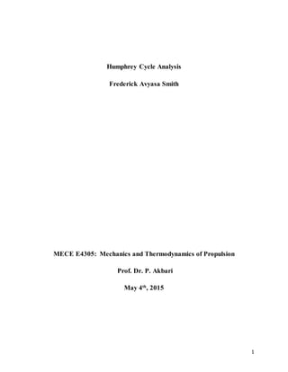
6. 6
Figure 1 Thermal Efficiency vs Compressor Pressure Ratio for Ideal Humphrey and Brayton Thermodynamic
Cycles with Varying 𝝉 𝟑 Values
It can be seen from Figure 1 that the Humphrey Cycle is always more efficient. It is noted that
Figure 1 was generated by finding τ4 using T1=288K, (4), and (5). Furthermore, Figure 1 was
generated by using (6) and (7).
Section B
In order to begin finding an expression for non-dimensional net work output in terms of τ4 and πc
we will use the expression for net work in a thermodynamic cycle and conservation of energy. It
is noted that this expression for net work applies directly to the Humphrey Cycle. We achieve:
𝑤 𝑛𝑒𝑡 = 𝐶 𝑣( 𝑇3 − 𝑇2) − 𝐶 𝑝( 𝑇4 − 𝑇1) (8)
Rearranging terms:
𝑤 𝑛𝑒𝑡
𝐶 𝑣 𝑇1
=
𝑇2
𝑇1
(
𝑇3
𝑇2
− 1) − 𝑘( 𝜏4 − 1) (9)
Using (4) and (5):
𝑤 𝑛𝑒𝑡
𝐶 𝑣 𝑇1
= 𝜋𝑐
𝑘−1
𝑘 ( 𝜏4
𝑘
− 1) − 𝑘( 𝜏4 − 1) (10)
By using the same method to find T4 as in Section A we can plot non-dimensional work output in
terms of τ4 and πc:
7. 7
Figure 2 Non-Dimensional Net Work vs Compressor Pressure Ratio for Ideal Humphrey Thermodynamic Cycle
with Varying 𝝉 𝟑 Values
It is noted Figure 2 was generated using (10).
Section C
In order to find thermal efficiency in terms of τ3 and πc we will utilize (3). Combining with (4)
and (5) and simplifying we achieve:
𝜂𝑡ℎ,ℎ = 1 −
𝑘𝜋𝑐
−𝑘+1
𝑘 (𝜏3
𝑘−1
𝜋𝑐
−𝑘+1
𝑘2
− 1)
𝜏3 𝜋𝑐
−𝑘+1
𝑘 − 1
(11)
To find non-dimensional net work in terms of τ3 and πc we will utilize (9). Again combining with
(4) and (5) then simplifying we achieve:
𝑊𝑛𝑒𝑡
𝐶 𝑣 𝑇1
= 𝜋𝑐
𝑘−1
𝑘 (𝜏3 𝜋𝑐
−𝑘+1
𝑘 − 1) − 𝑘 (𝜏3
𝑘−1
𝜋𝑐
−𝑘+1
𝑘2
− 1)(12)
Below one can find plots for both thermal efficiency and non-dimensional network:
8. 8
Figure 3 Thermal Efficiency vs Compressor Pressure Ratio for Ideal Humphrey Thermodynamic Cycle with
Varying 𝝉 𝟑 Values
Figure 4 Non-Dimensional Net Work vs Compressor Pressure Ratio for Ideal Humphrey Thermodynamic Cycle
with Varying 𝝉 𝟑 Values
It is noted that Figure 3 and Figure 4 were generated using (11) and (12).
From Figure 3 one can see that as πc increases thermal efficiency increases as well. This is to be
expected, as it is known that higher temperatures in a thermodynamic cycle will increase thermal
efficiency. This is the same reason why efficiency is greater in the figure for higher τ3 values.
When fixing τ3 and increasing πc thermal efficiency still increases because of the definition of
thermal efficiency in a thermodynamic cycle, however net work decreases. As one may envision
9. 9
from a T-S diagram with a fixed T3 value the area between the heat addition/rejection curves
diminished until it becomes zero. Thus, in an ideal cycle scenario there is a specific thermal
efficiency value where net work will equal zero. When τ3 is not fixed T3 may be increased thus
leading to not only increased efficiencies but also increased net work. In reality T3 is a highly
controlled parameter because of structural concerns relating to the turbine.
From Figure 4 it can be seen that there are πc values for maximum net work. As previously
discussed as τ3 increases so does T3, thus increasing net work. Thus, for higher τ3 values the
maximum net work value is increased. In addition as previously discussed net work decreases
with increasing πc . As T2 approaches T3 because of πc the area inside the heat addition/rejection
curves, in the cycles T-S diagram, shrinks indicating a loss in net work. Finally as T2 nears T3 the
area is reduced to zero, as there is no heat addition. Figure 4 clearly indicates that there is a
maximum πc value where net work becomes zero.
Section D
There is no explicit term for optimal πc that maximizes thermal efficiency. Like an ideal Brayton
Cycle thermal efficiency increases with πc for an ideal Humphrey Cycle. Eventually at very high
πc’s T2 approaches T3 meaning no heat is added to the thermodynamic cycle. With no heat added
to the cycle no work is generated. This defeats the purpose of a propulsion system. The πc when
zero net work is generated can be described as the maximum πc. At this point thermal efficiency
is also at its highest possible value, while propulsion is still being generated. Thus at maximum
πc thermal efficiency is also at its maximum.
In order to find a πc value for maximum thermal efficiency we will determine an expression for
maximum πc. By using the expression for non-dimensional net work, (12), and setting to zero we
achieve:
0 = 𝜋𝑐
𝑘−1
𝑘 (𝜏3 𝜋𝑐
−𝑘+1
𝑘 − 1) − 𝑘 (𝜏3
𝑘−1
𝜋𝑐
−𝑘+1
𝑘 − 1)(13)
By solving for πc we achieve:
𝜋𝑐,𝑚𝑎𝑥 = 𝜏3
𝑘
𝑘−1 − 𝑘
2
𝑘−1 − 𝑘
2
𝑘−1 𝜏3
−𝑘+1
𝜋𝑐,𝑚𝑎𝑥
−𝑘+1
𝑘2−𝑘 (14)
By solving for this equation numerically one can find a value for maximum πc, which equals the
πc that maximizes thermal efficiency.
10. 10
In order to determine an expression for the thermal efficiency, which results from maximum πc,
we can simply insert the term πc,max into expression (11). This results in:
𝜂𝑡ℎ,ℎ,𝑚𝑎𝑥 = 1 −
𝑘𝜋𝑐,𝑚𝑎𝑥
−𝑘+1
𝑘 (𝜏3
𝑘−1
𝜋𝑐,𝑚𝑎𝑥
−𝑘+1
𝑘2
− 1)
𝜏3 𝜋𝑐,𝑚𝑎𝑥
−𝑘+1
𝑘 − 1
(15)
One can interpret this point using graphs that include non-dimensional net work vs πc and
thermal efficiency vs πc. By locating the πc when non-dimensional net work becomes zero one
can locate the maximum thermal efficiency value by using the same πc.
Section E
In order to find expression for thermal efficiency and non-dimensional net work in terms of τ3,
πc, ηc, ηt and k we will begin by using the definition of compressor efficiency:
𝜂 𝑐 =
𝑊𝑖𝑠𝑒𝑛𝑡𝑟𝑜𝑝𝑖𝑐
𝑊𝑎𝑐𝑡𝑢𝑎𝑙
(16)
Using conservation of energy and simplifying we achieve:
𝜂 𝑐 =
𝑇2 − 𝑇1
𝑇2
′
− 𝑇1
(17)
Rearranging terms we can also achieve:
𝑇2
′
𝑇1
=
𝜂 𝑐 + ( 𝑇2
𝑇1
− 1)
𝜂𝑐
(18)
The same steps will be taken for turbine efficiency:
𝜂𝑡 =
𝑊𝑎𝑐𝑡𝑢𝑎𝑙
𝑊𝑖𝑠𝑒𝑛𝑡𝑟𝑜𝑝𝑖𝑐
(19)
𝜂𝑐 =
𝑇3 − 𝑇4
′
𝑇3 − 𝑇4
(20)
𝑇4
′
𝑇1
= 𝜏3 − 𝜂𝑡 (𝜏3 −
𝑇1
𝑇2
𝑘−1
𝜏3
𝑘−1
)(21)
By using (2) in terms of a cycle with irreversibilities and simplifying we begin to achieve an
expression for thermal efficiency with irreversibilities:
𝜂𝑡ℎ,ℎ = 1 −
𝑘 ( 𝑇4
′
𝑇1
− 1)
(𝜏3 − 𝑇2
′
𝑇1
)
(22)
After inserting (5), (18), (21), and simplifying we can obtain:
11. 11
𝜂𝑡ℎ,ℎ,𝑖 = 1 −
𝑘 [𝜏3 − 𝜂𝑡 (𝜏3 − 𝜏3
𝑘−1
𝜋𝑐
−𝑘+1
𝑘2
) − 1]
𝜏3 − 𝜂𝑐
−1 [𝜂𝑐 + (𝜋𝑐
𝑘−1
𝑘 − 1)]
(23)
Similarly using (9) in terms of a cycle with irreversibilities and simplifying we begin to achieve
an expression for non-dimensional net work with irreversibilities:
𝑤 𝑛𝑒𝑡
𝐶 𝑣 𝑇1
=
𝑇2
′
𝑇1
(
𝜏3
𝑇2
′
𝑇1
− 1) − 𝑘 (
𝑇4
′
𝑇1
− 1) (24)
Again after plugging in (5), (18), (21), and simplifying we can obtain:
𝑤 𝑛𝑒𝑡
𝐶 𝑣 𝑇1 𝑖
= 𝜂 𝑐
−1
[𝜂𝑐 + (𝜋𝑐
𝑘−1
𝑘 − 1)] [𝜏3 (𝜂 𝑐
−1
(𝜂𝑐 + (𝜋𝑐
𝑘−1
𝑘 − 1)))
−1
− 1]
− 𝑘 [𝜏3 − 𝜂𝑡 (𝜏3 − 𝜏3
𝑘−1
𝜋𝑐
−𝑘+1
𝑘2
) − 1] (25)
By setting ηc and ηt in (23) and (25) to 1 and rearranging terms equations (11) and (12) can be
found which are ideal expressions. This is a quick way to verify the validity of the expressions.
Below one can find plots for both thermal efficiency and non-dimensional network:
Figure 5 Thermal Efficiency vs Compressor Pressure Ratio For Ideal and Non-Ideal Humphrey Thermodynamic
Cyles with Varying 𝝉 𝟑 values
12. 12
Figure 6 Non-Dimensional Net Work vs Compressor Pressure Ratio for Ideal and Non-Ideal Humphrey
Thermodynamic Cycles with Varying 𝝉 𝟑 values
It is noted that Figure 5 and Figure 6 were generated using (23) and (25).
From Figure 5 one can see the effects of adding losses from the compressor and turbine. One
initially can see that the thermal efficiencies for each set of τ3’s across increasing πc’s for non-
ideal cycles are lower than the ideal cycles. In addition to this when losses are taken into account
thermal efficiencies do not keep climbing. It can be seen that there are maximum thermal
efficiency points for each fixed τ3’s at corresponding πc’s. Maximum thermal efficiency points
climb with increased τ3’s due to higher cycle temperatures, which provide better thermal
efficiency. In addition to this these points occur at higher πc’s for higher τ3’s because of the
needed T2 to reach necessary T3. After these maximum thermal efficiency points the values
begin to drop. The reductions in efficiencies are caused by the work needed to drive the
compressor. Just as maximum thermal efficiency points occur at lower πc’s for lower τ3’s, zero
thermal efficiency points occur at earlier πc’s for lower τ3’s.
From Figure 6 one can see the effects of adding losses from the compressor and turbine in regard
to non-dimensional net work. Initially one can see that the non-dimensional net work values are
significantly lower than the ideal cycles. This implies that maximum non-dimensional values are
also lower than the ideal cycles. Despite all values being significantly lower the behavior of the
cycles with losses greatly resemble the behavior of the ideal cycles. The only discrepancies are
13. 13
the increased slopes in the non-ideal cycles compared to the ideal cycles. As expected adding
losses form the compressor and turbine greatly reduce net work.
14. 14
References
1) Kamiuto, K. "Comparison of Basic Gas Cycles under the Restriction of Constant Heat
Addition." Science Direct. 1 Sept. 2005. Web. 3 May 2015.
<http://www.sciencedirect.com.ezproxy.cul.columbia.edu/science/article/pii/S030626190500085
1#>
2) Farokhi, Saeed. Aircraft Propulsion. Second ed. Chichester: John Wiley & Sons, 2014. Print.