The document describes three experiments conducted on student data from AlQadi University to predict student performance. The first used a random tree algorithm and produced a decision tree with over 150 nodes. The second used a W-LADTree algorithm and produced a tree with 31 nodes, 21 predictor nodes, and 13 leaves. The third used a J48 algorithm, which is based on decision tree induction and employs two pruning methods.

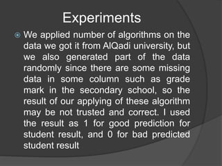
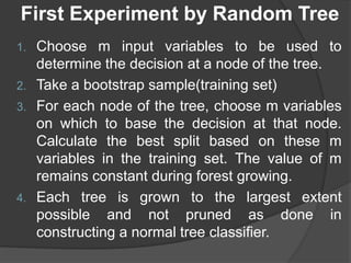
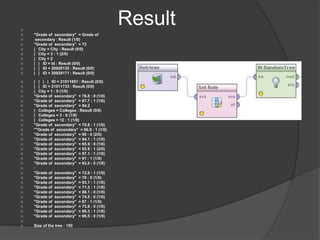
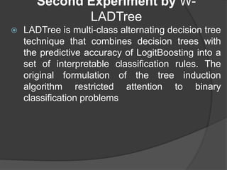
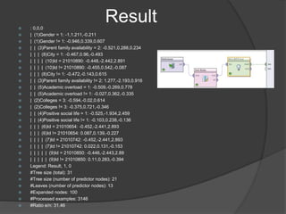
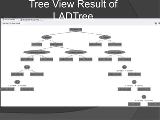
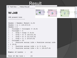
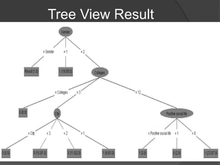
1. Prepared by
Mohammed Kharma

2. Impact of university
students social status on
their selection of academic
specialization and their
performance

3. Top 11 Factors extracted
 College
 Specialization
 Gender
 Grade of secondary
 Parent family availability: Student how have one
parent family or two parent family.
 If the student has job or not
 Financial aids, if he got a loan for his semester.
 Educational level of parents.
 Geographical location.
 Positive social life
 Academic overload

4. Experiments
 We applied number of algorithms on the
data we got it from AlQadi university, but
we also generated part of the data
randomly since there are some missing
data in some column such as grade
mark in the secondary school, so the
result of our applying of these algorithm
may be not trusted and correct. I used
the result as 1 for good prediction for
student result, and 0 for bad predicted
student result

5. Data Processing
The data used for each attribute are Classified as below:
Every table from the following describe the expected
labels for the identified attributes, for example the
first attribute “college” may has one of the 2 value
listed in “Attribute 1: College” table below
Attribute 1: College
12 Pharmacy
3 Science and Technology
Gender
1 Male
2 Female
Educational level of parents
2 High
1 Low
*High - over Secondary
*Low - Secondary or Less

6. Data Processing
has job
1 Has Job
0 No
Specialization
0305 Math
1201 Pharmacy
0302 Physics
City
1 Ramallah
2 Hebron
3 Jeneen
Parent family availability
2 Both
1 one of them
0 None

7. Data Processing
Positive social life
0 Positive
1 Negative
*Positive - Good and Stable Social Life
*Negative - Good and Stable Social Life
Academic overload
0 High
1 Low
*High - 15 Hour Or Greater
*Low - Less Than 15 Hour
Financial aids
1 Has aid
0 No
*Has aid - Student got financial Aid
*No aid - Student didn't got financial Aid

8. First Experiment by Random Tree
1. Choose m input variables to be used to
determine the decision at a node of the tree.
2. Take a bootstrap sample(training set)
3. For each node of the tree, choose m variables
on which to base the decision at that node.
Calculate the best split based on these m
variables in the training set. The value of m
remains constant during forest growing.
4. Each tree is grown to the largest extent
possible and not pruned as done in
constructing a normal tree classifier.

9. Result
 "Grade of secondary" = Grade of
 secondary : Result (1/0)
 "Grade of secondary" = 72
 | City = City : Result (0/0)
 | City = 3 : 1 (2/0)
 | City = 2
 | | ID = Id : Result (0/0)
 | | ID = 20920135 : Result (0/0)
 | | ID = 20920171 : Result (0/0)
○ :
 | | | | ID = 21011651 : Result (0/0)
 | | ID = 21011733 : Result (0/0)
 | City = 1 : 0 (1/0)
 "Grade of secondary" = 76.8 : 0 (1/0)
 "Grade of secondary" = 87.7 : 1 (1/0)
 "Grade of secondary" = 94.2
 | Colleges = Colleges : Result (0/0)
 | Colleges = 3 : 0 (1/0)
 | Colleges = 12 : 1 (1/0)
 "Grade of secondary" = 70.8 : 1 (1/0)
 ""Grade of secondary" = 86.9 : 1 (1/0)
 "Grade of secondary" = 90 : 0 (2/0)
 "Grade of secondary" = 94.1 : 1 (1/0)
 "Grade of secondary" = 95.9 : 0 (1/0)
 "Grade of secondary" = 92.9 : 1 (2/0)
 "Grade of secondary" = 97.1 : 1 (1/0)
 "Grade of secondary" = 91 : 1 (1/0)
 "Grade of secondary" = 93.4 : 0 (1/0)
 :
 "Grade of secondary" = 72.9 : 1 (1/0)
 "Grade of secondary" = 78 : 0 (1/0)
 "Grade of secondary" = 93.1 : 1 (1/0)
 "Grade of secondary" = 71.2 : 1 (1/0)
 "Grade of secondary" = 88.1 : 0 (1/0)
 "Grade of secondary" = 74.5 : 0 (1/0)
 "Grade of secondary" = 87 : 1 (1/0)
 "Grade of secondary" = 73.8 : 0 (1/0)
 "Grade of secondary" = 86.3 : 1 (1/0)
 "Grade of secondary" = 96.5 : 0 (1/0)

 Size of the tree : 150

10. Second Experiment by W-
LADTree
 LADTree is multi-class alternating decision tree
technique that combines decision trees with
the predictive accuracy of LogitBoosting into a
set of interpretable classification rules. The
original formulation of the tree induction
algorithm restricted attention to binary
classification problems

11. Result : 0,0,0
 | (1)Gender = 1: -1,1.211,-0.211
 | (1)Gender != 1: -0.946,0.339,0.607
 | | (3)Parent family availability = 2: -0.521,0.288,0.234
 | | | (8)City = 1: -0.467,0.96,-0.493
 | | | | (10)Id = 21010890: -0.448,-2.442,2.891
 | | | | (10)Id != 21010890: -0.455,0.542,-0.087
 | | | (8)City != 1: -0.472,-0.143,0.615
 | | (3)Parent family availability != 2: 1.277,-2.193,0.916
 | | (5)Academic overload = 1: -0.509,-0.269,0.778
 | | (5)Academic overload != 1: -0.027,0.362,-0.335
 | (2)Colleges = 3: -0.594,-0.02,0.614
 | (2)Colleges != 3: -0.375,0.721,-0.346
 | | (4)Positive social life = 1: -0.525,-1.934,2.459
 | | (4)Positive social life != 1: -0.103,0.238,-0.136
 | | | (6)Id = 21010654: -0.452,-2.441,2.893
 | | | (6)Id != 21010654: 0.087,0.139,-0.227
 | | | | (7)Id = 21010742: -0.452,-2.441,2.893
 | | | | (7)Id != 21010742: 0.022,0.131,-0.153
 | | | | | (9)Id = 21010850: -0.446,-2.443,2.89
 | | | | | (9)Id != 21010850: 0.11,0.283,-0.394
 Legend: Result, 1, 0
 #Tree size (total): 31
 #Tree size (number of predictor nodes): 21
 #Leaves (number of predictor nodes): 13
 #Expanded nodes: 100
 #Processed examples: 3146
 #Ratio e/n: 31.46

12. Tree View Result of
LADTree

13. Third Experiment by W-J48
 J48 Is a standard algorithm in machine learning
based on decision tree induction, this algorithm
employs two pruning methods. In the first method
“sub-tree replacement”, the nodes in a decision
tree may be replaced with a leaf to reducing the
number of tests along a specific path. The steps of
algorithm are:
 Algorithm starts from the leaves of the fully formed
tree and works backwards the root to reduce
number of test along the path. While in the second
type “sub-tree raising”, where a node may be
moved upwards the root of the tree, replacing
other nodes along the path. Sub-tree raising
usually has a effect on decision tree models.

14. Result

15. Tree View Result

16. -Thank you