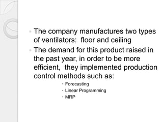
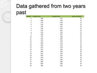
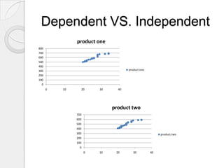
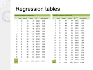
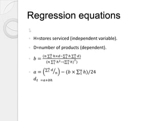
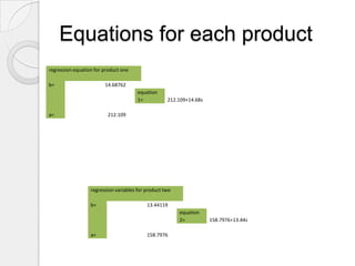
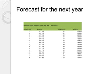
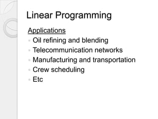
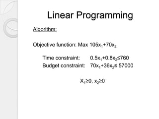
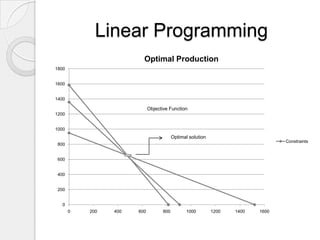
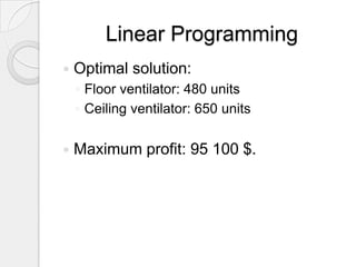
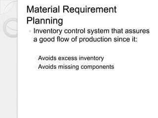
A production example


           Ramon Savinon
           Sophie Leroux 1939653
           Stephanie Soares
                  9764925
Introduction
 The base of the model is a fictional
  company located in the Dominican
  Republic
 Its headquarters is located in Santo
  Domingo, and it supplies appliances
  stores in 3 main cities
   Lead factors:
     High cost of electricity
     Humidity factor is very high
 The company manufactures two types
  of ventilators: floor and ceiling
 The demand for this product raised in
  the past year, in order to be more
  efficient, they implemented production
  control methods such as:
           Forecasting
           Linear Programming
           MRP
Forecasting
   The forescating method used was a
    type of regression called linear
    regression. It tries to evaluate the
    correlation beetween two variables.
Data gathered from two years
past
    Period    product one         product two         stores serviced
          1                 500                 411                 20
          2                 508                 416                 21
          3                 514                 430                 21
          4                 518                 430                 21
          5                 518                 431                 22
          6                 534                 456                 22
          7                 535                 461                 22
          8                 553                 463                 23
          9                 558                 477                 24
         10                 573                 486                 25
         11                 576                 487                 25
         12                 579                 504                 25
         13                 584                 514                 25
         14                 585                 533                 26
         15                 591                 539                 26
         16                 621                 544                 28
         17                 646                 546                 28
         18                 661                 563                 28
         19                 663                 563                 28
         20                 674                 576                 29
         21                 681                 585                 32
         22                 684                 589                 34
         23                 689                 589                 34
         24                 696                 592                 34
Dependent VS. Independent
               product one
800
700
600
500
400
300                                  product one
200
100
  0
      0   10     20      30     40


                              product two
               700
               600
               500
               400
               300                                      product two
               200
               100
                 0
                     0   10    20       30         40
Regression tables
regression computation for product one                            regression computation for product two
                                          demand                                                            demand
t        stores    demand     store^2     ^2      stores*demand   t        stores    demand     store^2     ^2        stores*demand
     1        20        500         400    250000   10000              1        20        411         400    168921       8220
     2        21        508         441    258064   10668              2        21        416         441    173056       8736
     3        21        514         441    264196   10794              3        21        430         441    184900       9030
     4        21        518         441    268324   10878              4        21        430         441    184900       9030
     5        22        518         484    268324   11396              5        22        431         484    185761       9482
     6        22        534         484    285156   11748              6        22        456         484    207936      10032
     7        22        535         484    286225   11770              7        22        461         484    212521      10142
     8        23        553         529    305809   12719              8        23        463         529    214369      10649
     9        24        558         576    311364   13392              9        24        477         576    227529      11448
    10        25        573         625    328329   14325
                                                                      10        25        486         625    236196      12150
    11        25        576         625    331776   14400
                                                                      11        25        487         625    237169      12175
    12        25        579         625    335241   14475
                                                                      12        25        504         625    254016      12600
    13        25        584         625    341056   14600
                                                                      13        25        514         625    264196      12850
    14        26        585         676    342225   15210
                                                                      14        26        533         676    284089      13858
    15        26        591         676    349281   15366
                                                                      15        26        539         676    290521      14014
    16        28        621         784    385641   17388
                                                                      16        28        544         784    295936      15232
    17        28        646         784    417316   18088
                                                                      17        28        546         784    298116      15288
    18        28        661         784    436921   18508
    19        28        663         784    439569   18564             18        28        563         784    316969      15764
    20        29        674         841    454276   19546             19        28        563         784    316969      15764
    21        32        681        1024    463761   21792             20        29        576         841    331776      16704
    22        34        684        1156    467856   23256             21        32        585        1024    342225      18720
    23        34        689        1156    474721   23426             22        34        589        1156    346921      20026
    24        34        696        1156    484416   23664             23        34        589        1156    346921      20026
                                                                      24        34        592        1156    350464      20128
total       623       14241      16601    8549847   375973
                                                                  total       623       12185       16601   6272377    322068
Regression equations

Equations for each product
regression equation for product one

b=                      14.68762
                                       equation
                                       1=           212.109+14.68s

a=                       212.109


                  regression variables for product two

                  b=                       13.44119
                                                         equation
                                                         2=          158.7976+13.44s

                  a=                       158.7976
Forecast for the next year

  expected stores to service in the next year   per month

  product one           forecast                            product two   forecast
          27               517.469                                  26           508.23
          25               488.109                                  26           508.23
          30               561.509                                  28           535.11
          26               502.789                                  28           535.11
          26               502.789                                  25           494.79
          25               488.109                                  29           548.55
          28               532.149                                  30           561.99
          30               561.509                                  30           561.99
          28               532.149                                  30           561.99
          28               532.149                                  29           548.55
          26               502.789                                  27           521.67
          29               546.829                                  25           494.79
          30               561.509                                  28           535.11
Linear Programming
 Linear Programming is a specific class
  of mathematical problems.
 It was first used during the First World
  War to solve complex problems in
  warfare.
 Later on, it was developed by George
  B. Dantzig, who is regarded as the
  father of LP.
Linear Programming
Applications
 Oil refining and blending
 Telecommunication networks
 Manufacturing and transportation
 Crew scheduling
 Etc
Linear Programming
Algorithm:

Objective function: Max 105x1+70x2

    Time constraint:   0.5x1+0.8x2≤760
    Budget constraint: 70x1+36x2≤ 57000

                   X1≥0, x2≥0
To solve this problem, LINDO was
 used.

LINDO is a software that is frequently
  used to solve linear and non linear
  problems.
Linear Programming
                         Optimal Production
1800


1600


1400

                             Objective Function
1200


1000
                                          Optimal solution
                                                                                  Constraints
 800


 600


 400


 200


   0
       0   200   400   600          800          1000        1200   1400   1600
Linear Programming
   Optimal solution:
    ◦ Floor ventilator: 480 units
    ◦ Ceiling ventilator: 650 units

   Maximum profit: 95 100 $.
Material Requirement
Planning
   Inventory control system that assures
    a good flow of production since it:

    ◦ Avoids excess inventory
    ◦ Avoids missing components
Material Requirement
Planning
   MRP suggests ordering schedule
    providing:
    ◦ Quantities
    ◦ Time of ordering (leading time)

» In order for a certain number of
 products to be ready at a given time.
Material Requirement
Planning
Important considerations:
 Quantities (product structure diagrams)
 Lead time
 Lot sizes: Lot sizes might not be equal to
  the needed quantity, resulting in
  exceeding inventory. The MRP, when
  used on a weekly basis, includes these
  values in the calculations to ensure a
  good utilization of the stock and avoid
  financial and material loss.
Material Requirement
Planning
Applying MRP to our problem:
 From linear programming, we found
  optimal monthly production values for
  each product:

Product 1 : 480 units (ie: 480 units need to be ready
  by the end of week 4).
Product 2 : 650 units

***Assuming lot size of 100 for all components and
  subassemblies
Material Requirement
Planning
   Product Structure Diagram for Product
    1 (floor ventilators)

                                         Product 1


                      SA 1                                      SA 2
                 (1unit/product)                           (2 units/prod.)


             C1                                       C3                   C4
                                  C2
              (1                                       (1                   (1
                            (2 units/prod.)
        unit/product)                            unit/product)        unit/product)
Material Requirement
Planning
   Product Structure Diagram for Product
    2 (ceiling ventilators)

                                    Product 2


                        SA 1
                                                     SA 2
                          (1
                                                (2 units/prod.)
                    unit/product)


               C1
                                   C2                C3
                (1
                             (2 units/prod.)    (2 units/prod)
          unit/product)
Feel free to ask questions...
Thank you for your attention!!

Production Engineering Principles

  • 1.
    A production example Ramon Savinon Sophie Leroux 1939653 Stephanie Soares 9764925
  • 2.
    Introduction  The baseof the model is a fictional company located in the Dominican Republic  Its headquarters is located in Santo Domingo, and it supplies appliances stores in 3 main cities
  • 3.
    Lead factors:  High cost of electricity  Humidity factor is very high
  • 4.
     The companymanufactures two types of ventilators: floor and ceiling  The demand for this product raised in the past year, in order to be more efficient, they implemented production control methods such as:  Forecasting  Linear Programming  MRP
  • 5.
    Forecasting  The forescating method used was a type of regression called linear regression. It tries to evaluate the correlation beetween two variables.
  • 6.
    Data gathered fromtwo years past Period product one product two stores serviced 1 500 411 20 2 508 416 21 3 514 430 21 4 518 430 21 5 518 431 22 6 534 456 22 7 535 461 22 8 553 463 23 9 558 477 24 10 573 486 25 11 576 487 25 12 579 504 25 13 584 514 25 14 585 533 26 15 591 539 26 16 621 544 28 17 646 546 28 18 661 563 28 19 663 563 28 20 674 576 29 21 681 585 32 22 684 589 34 23 689 589 34 24 696 592 34
  • 7.
    Dependent VS. Independent product one 800 700 600 500 400 300 product one 200 100 0 0 10 20 30 40 product two 700 600 500 400 300 product two 200 100 0 0 10 20 30 40
  • 8.
    Regression tables regression computationfor product one regression computation for product two demand demand t stores demand store^2 ^2 stores*demand t stores demand store^2 ^2 stores*demand 1 20 500 400 250000 10000 1 20 411 400 168921 8220 2 21 508 441 258064 10668 2 21 416 441 173056 8736 3 21 514 441 264196 10794 3 21 430 441 184900 9030 4 21 518 441 268324 10878 4 21 430 441 184900 9030 5 22 518 484 268324 11396 5 22 431 484 185761 9482 6 22 534 484 285156 11748 6 22 456 484 207936 10032 7 22 535 484 286225 11770 7 22 461 484 212521 10142 8 23 553 529 305809 12719 8 23 463 529 214369 10649 9 24 558 576 311364 13392 9 24 477 576 227529 11448 10 25 573 625 328329 14325 10 25 486 625 236196 12150 11 25 576 625 331776 14400 11 25 487 625 237169 12175 12 25 579 625 335241 14475 12 25 504 625 254016 12600 13 25 584 625 341056 14600 13 25 514 625 264196 12850 14 26 585 676 342225 15210 14 26 533 676 284089 13858 15 26 591 676 349281 15366 15 26 539 676 290521 14014 16 28 621 784 385641 17388 16 28 544 784 295936 15232 17 28 646 784 417316 18088 17 28 546 784 298116 15288 18 28 661 784 436921 18508 19 28 663 784 439569 18564 18 28 563 784 316969 15764 20 29 674 841 454276 19546 19 28 563 784 316969 15764 21 32 681 1024 463761 21792 20 29 576 841 331776 16704 22 34 684 1156 467856 23256 21 32 585 1024 342225 18720 23 34 689 1156 474721 23426 22 34 589 1156 346921 20026 24 34 696 1156 484416 23664 23 34 589 1156 346921 20026 24 34 592 1156 350464 20128 total 623 14241 16601 8549847 375973 total 623 12185 16601 6272377 322068
  • 9.
  • 10.
    Equations for eachproduct regression equation for product one b= 14.68762 equation 1= 212.109+14.68s a= 212.109 regression variables for product two b= 13.44119 equation 2= 158.7976+13.44s a= 158.7976
  • 11.
    Forecast for thenext year expected stores to service in the next year per month product one forecast product two forecast 27 517.469 26 508.23 25 488.109 26 508.23 30 561.509 28 535.11 26 502.789 28 535.11 26 502.789 25 494.79 25 488.109 29 548.55 28 532.149 30 561.99 30 561.509 30 561.99 28 532.149 30 561.99 28 532.149 29 548.55 26 502.789 27 521.67 29 546.829 25 494.79 30 561.509 28 535.11
  • 12.
    Linear Programming  LinearProgramming is a specific class of mathematical problems.  It was first used during the First World War to solve complex problems in warfare.  Later on, it was developed by George B. Dantzig, who is regarded as the father of LP.
  • 13.
    Linear Programming Applications  Oilrefining and blending  Telecommunication networks  Manufacturing and transportation  Crew scheduling  Etc
  • 14.
    Linear Programming Algorithm: Objective function:Max 105x1+70x2 Time constraint: 0.5x1+0.8x2≤760 Budget constraint: 70x1+36x2≤ 57000 X1≥0, x2≥0
  • 15.
    To solve thisproblem, LINDO was used. LINDO is a software that is frequently used to solve linear and non linear problems.
  • 16.
    Linear Programming Optimal Production 1800 1600 1400 Objective Function 1200 1000 Optimal solution Constraints 800 600 400 200 0 0 200 400 600 800 1000 1200 1400 1600
  • 17.
    Linear Programming  Optimal solution: ◦ Floor ventilator: 480 units ◦ Ceiling ventilator: 650 units  Maximum profit: 95 100 $.
  • 18.
    Material Requirement Planning  Inventory control system that assures a good flow of production since it: ◦ Avoids excess inventory ◦ Avoids missing components
  • 19.
    Material Requirement Planning  MRP suggests ordering schedule providing: ◦ Quantities ◦ Time of ordering (leading time) » In order for a certain number of products to be ready at a given time.
  • 20.
    Material Requirement Planning Important considerations: Quantities (product structure diagrams)  Lead time  Lot sizes: Lot sizes might not be equal to the needed quantity, resulting in exceeding inventory. The MRP, when used on a weekly basis, includes these values in the calculations to ensure a good utilization of the stock and avoid financial and material loss.
  • 21.
    Material Requirement Planning Applying MRPto our problem:  From linear programming, we found optimal monthly production values for each product: Product 1 : 480 units (ie: 480 units need to be ready by the end of week 4). Product 2 : 650 units ***Assuming lot size of 100 for all components and subassemblies
  • 22.
    Material Requirement Planning  Product Structure Diagram for Product 1 (floor ventilators) Product 1 SA 1 SA 2 (1unit/product) (2 units/prod.) C1 C3 C4 C2 (1 (1 (1 (2 units/prod.) unit/product) unit/product) unit/product)
  • 23.
    Material Requirement Planning  Product Structure Diagram for Product 2 (ceiling ventilators) Product 2 SA 1 SA 2 (1 (2 units/prod.) unit/product) C1 C2 C3 (1 (2 units/prod.) (2 units/prod) unit/product)
  • 24.
    Feel free toask questions...
  • 25.
    Thank you foryour attention!!