This document discusses the handling of missing data in pandas, explaining how to identify, fill, and remove missing values using various functions like isnull(), fillna(), and dropna(). It also covers reshaping dataframes, merging dataframes, and basic plotting techniques with matplotlib, providing examples for each method. Overall, it serves as a comprehensive guide for managing data and visualizations in Python's pandas library.

1. Missing Data Handling
Missing Data can occur when no information is provided for one or more items or for a
whole unit.
Missing Data is a very big problem in a real-life scenarios.
Missing Data can also refer to as NA(Not Available) values in pandas.
In DataFrame sometimes many datasets simply arrive with missing data, either because it
exists and was not collected or it never existed.
In Pandas missing data is represented by two value:
None: None is a Python singleton object that is often used for missing data in Python code.
NaN : NaN (an acronym for Not a Number)
Several useful functions for detecting, removing, and replacing null values in Pandas
DataFrame

2. Missing Data Handling
isnull()
notnull()
dropna()
fillna()
replace()
interpolate()
Checking for missing values using isnull() and notnull()
Both function help in checking whether a value is NaN or not
Checking for missing values using isnull()
In order to check null values in Pandas DataFrame, we use isnull() function this function
return dataframe of Boolean values which are True for NaN values.

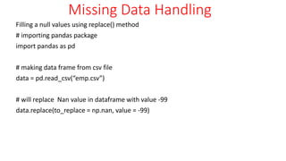
3. Missing Data Handling
# importing pandas as pd
import pandas as pd
# importing numpy as np
import numpy as np
# dictionary of lists
dict = {'First Score':[100, 90, np.nan, 95],
'Second Score': [30, 45, 56, np.nan],
'Third Score':[np.nan, 40, 80, 98]}
# creating a dataframe from list
df = pd.DataFrame(dict)
# using isnull() function
df.isnull()

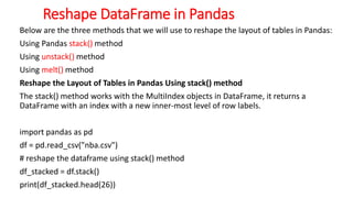
4. Missing Data Handling
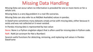
Checking for missing values using notnull()
In order to check null values in Pandas Dataframe, we use notnull() function this function return dataframe of
Boolean values which are False for NaN values.
import pandas as pd
import numpy as np
# dictionary of lists
dict = {'First Score':[100, 90, np.nan, 95],
'Second Score': [30, 45, 56, np.nan],
'Third Score':[np.nan, 40, 80, 98]}
# creating a dataframe using dictionary
df = pd.DataFrame(dict)
# using notnull() function
df.notnull()

5. Missing Data Handling
Filling missing values using fillna(), replace() and interpolate()
In order to fill null values in a datasets, we use fillna(), replace() and interpolate() function
these function replace NaN values with some value of their own.
All these function help in filling a null values in datasets of a DataFrame.
Interpolate() function is basically used to fill NA values in the dataframe but it uses various
interpolation technique to fill the missing values rather than hard-coding the value.

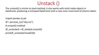
6. Missing Data Handling
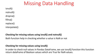
import pandas as pd
import numpy as np
# dictionary of lists
dict = {'First Score':[100, 90, np.nan, 95],
'Second Score': [30, 45, 56, np.nan],
'Third Score':[np.nan, 40, 80, 98]}
# creating a dataframe from dictionary
df = pd.DataFrame(dict)
# filling missing value using fillna()
df.fillna(0)

7. Missing Data Handling
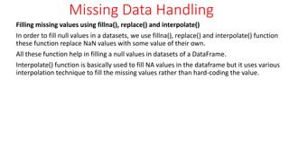
Filling null values with the previous ones
import pandas as pd
import numpy as np
dict = {'First Score':[100, 90, np.nan, 95],
'Second Score': [30, 45, 56, np.nan],
'Third Score':[np.nan, 40, 80, 98]}
df = pd.DataFrame(dict)
# filling a missing value with previous ones
df.fillna(method ='pad')

8. Missing Data Handling
Filling null value with the next ones
import pandas as pd
import numpy as np
dict = {'First Score':[100, 90, np.nan, 95],
'Second Score': [30, 45, 56, np.nan],
'Third Score':[np.nan, 40, 80, 98]}
df = pd.DataFrame(dict)
# filling null value using fillna() function
df.fillna(method ='bfill')

9. Missing Data Handling
Filling a null values using replace() method
# importing pandas package
import pandas as pd
# making data frame from csv file
data = pd.read_csv(“emp.csv”)
# will replace Nan value in dataframe with value -99
data.replace(to_replace = np.nan, value = -99)

10. Missing Data Handling
Using interpolate() function to fill the missing values using linear method.
# importing pandas as pd
import pandas as pd
# Creating the dataframe
df = pd.DataFrame({"A":[12, 4, 5, None, 1],
"B":[None, 2, 54, 3, None],
"C":[20, 16, None, 3, 8],
"D":[14, 3, None, None, 6]})
# Print the dataframe
df
df.interpolate(method ='linear', limit_direction ='forward')

11. Missing Data Handling
Dropping missing values using dropna()
In order to drop a null values from a dataframe, we used dropna() function this function
drop Rows/Columns of datasets with Null values in different ways.
import pandas as pd
import numpy as np
dict = {'First Score':[100, 90, np.nan, 95],
'Second Score': [30, np.nan, 45, 56],
'Third Score':[52, 40, 80, 98],
'Fourth Score':[np.nan, np.nan, np.nan, 65]}
df = pd.DataFrame(dict)
# using dropna() function
df.dropna()#df.dropna(how = 'all')

12. Reshape DataFrame in Pandas
Below are the three methods that we will use to reshape the layout of tables in Pandas:
Using Pandas stack() method
Using unstack() method
Using melt() method
Reshape the Layout of Tables in Pandas Using stack() method
The stack() method works with the MultiIndex objects in DataFrame, it returns a
DataFrame with an index with a new inner-most level of row labels.
import pandas as pd
df = pd.read_csv("nba.csv")
# reshape the dataframe using stack() method
df_stacked = df.stack()
print(df_stacked.head(26))

13. Unstack ()
The unstack() is similar to stack method, It also works with multi-index objects in
dataframe, producing a reshaped DataFrame with a new inner-most level of column labels.
import pandas as pd
df = pd.read_csv("nba.csv")
# unstack() method
df_unstacked = df_stacked.unstack()
print(df_unstacked.head(10))

14. Melt()
The melt() in Pandas reshape dataframe from wide format to long format.
It uses the “id_vars[‘col_names’]” to melt the dataframe by column names.
import pandas as pd
df = pd.read_csv("nba.csv")
# it takes two columns "Name" and "Team"
df_melt = df.melt(id_vars=['Name', 'Team'])
print(df_melt.head(10))

15. Merge, join, concatenate and compare
concat(): Merge multiple Series or DataFrame objects along a shared index or column
DataFrame.join(): Merge multiple DataFrame objects along the columns
merge(): Combine two Series or DataFrame objects with SQL-style joining
merge_ordered(): Combine two Series or DataFrame objects along an ordered axis
Series.compare() and DataFrame.compare(): Show differences in values between two
Series or DataFrame objects

16. concat()
The concat() function concatenates an arbitrary amount of Series or DataFrame objects along an axis while performing optional set logic (union or intersection) of the
indexes on the other axes.
Like numpy.concatenate, concat() takes a list or dict of homogeneously-typed objects and concatenates them.
import pandas as pd
df1 = pd.DataFrame(
{
"A": ["A0", "A1", "A2", "A3"],
"B": ["B0", "B1", "B2", "B3"],
"C": ["C0", "C1", "C2", "C3"],
"D": ["D0", "D1", "D2", "D3"],
},
index=[0, 1, 2, 3],)
df2 = pd.DataFrame(
{
"A": ["A4", "A5", "A6", "A7"],
"B": ["B4", "B5", "B6", "B7"],
"C": ["C4", "C5", "C6", "C7"],
"D": ["D4", "D5", "D6", "D7"],
},
index=[4, 5, 6, 7],)
frames = [df1, df2]
result = pd.concat(frames)
print(result)

17. Join()
The join keyword specifies how to handle axis values that don’t exist in the first DataFrame.
join='outer' takes the union of all axis values
import pandas as pd
df1 = pd.DataFrame(
{
"A": ["A0", "A1", "A2", "A3"],
"B": ["B0", "B1", "B2", "B3"],
"C": ["C0", "C1", "C2", "C3"],
"D": ["D0", "D1", "D2", "D3"],
},
index=[0, 1, 2, 3],)
df2 = pd.DataFrame(
{
"A": ["A4", "A5", "A6", "A7"],
"B": ["B4", "B5", "B6", "B7"],
"C": ["C4", "C5", "C6", "C7"],
"D": ["D4", "D5", "D6", "D7"],
},
index=[4, 5, 6, 7],)
frames = [df1, df2]
result = pd.concat(frames)

18. df4 = pd.DataFrame(
{
"B": ["B2", "B3", "B6", "B7"],
"D": ["D2", "D3", "D6", "D7"],
"F": ["F2", "F3", "F6", "F7"],
},
index=[2, 3, 6, 7],
)
result = pd.concat([df1, df4], axis=1)
print(result)

19. Series and DataFrame Join
import pandas as pd
df1 = pd.DataFrame(
{
"A": ["A0", "A1", "A2", "A3"],
"B": ["B0", "B1", "B2", "B3"],
"C": ["C0", "C1", "C2", "C3"],
"D": ["D0", "D1", "D2", "D3"],
},
index=[0, 1, 2, 3],)
s1 = pd.Series(["X0", "X1", "X2", "X3"], name="X")
result = pd.concat([df1, s1], axis=1)
print(result)

20. merge()
merge() performs join operations similar to relational databases like SQL. Users who are
familiar with SQL but new to pandas can reference a comparison with SQL.
Merge types
merge() implements common SQL style joining operations.
one-to-one: joining two DataFrame objects on their indexes which must contain unique
values.
many-to-one: joining a unique index to one or more columns in a different DataFrame.
many-to-many : joining columns on columns.

21. import pandas as pd
left = pd.DataFrame(
{
"key": ["K0", "K1", "K2", "K3"],
"A": ["A0", "A1", "A2", "A3"],
"B": ["B0", "B1", "B2", "B3"],
}
)
right = pd.DataFrame(
{
"key": ["K0", "K1", "K2", "K3"],
"C": ["C0", "C1", "C2", "C3"],
"D": ["D0", "D1", "D2", "D3"],
}
)
result = pd.merge(left, right, on="key")
print(result)

22. Merge method SQL Join Name Description
left LEFT OUTER JOIN Use keys from left
frame only
right RIGHT OUTER JOIN Use keys from right
frame only
outer FULL OUTER JOIN Use union of keys
from both frames
inner INNER JOIN Use intersection of
keys from both frames
cross CROSS JOIN Create the cartesian
product of rows of
both frames

23. Import pandas as pd
left = pd.DataFrame(
{
"key1": ["K0", "K0", "K1", "K2"],
"key2": ["K0", "K1", "K0", "K1"],
"A": ["A0", "A1", "A2", "A3"],
"B": ["B0", "B1", "B2", "B3"],
}
)
right = pd.DataFrame(
{
"key1": ["K0", "K1", "K1", "K2"],
"key2": ["K0", "K0", "K0", "K0"],
"C": ["C0", "C1", "C2", "C3"],
"D": ["D0", "D1", "D2", "D3"],
}
)
result = pd.merge(left, right, how="left", on=["key1", "key2"])
result

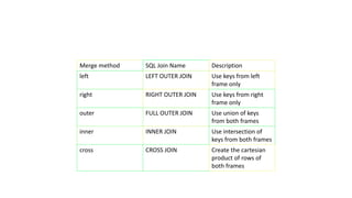
24. result = pd.merge(left, right, how="right", on=["key1", "key2"])
print(result)
result = pd.merge(left, right, how="outer", on=["key1", "key2"])
print(result)
result = pd.merge(left, right, how="inner", on=["key1", "key2"])
print(result)
result = pd.merge(left, right, how="cross")
print(result)

25. • S.min()
• S.max()
• S.sum()
• Describe
• Head()
• Tail()
• Data[column].diff().head()

26. PLOTTING
Plotting x and y points
The plot() function is used to draw points (markers) in a diagram.
By default, the plot() function draws a line from point to point.
The function takes parameters for specifying points in the diagram.
Parameter 1 is an array containing the points on the x-axis.
Parameter 2 is an array containing the points on the y-axis.
If we need to plot a line from (1, 3) to (8, 10), we have to pass two arrays [1, 8]
and [3, 10] to the plot function.

27. import matplotlib.pyplot as plt
import numpy as np
xpoints = np.array([1, 8])
ypoints = np.array([3, 10])
plt.plot(xpoints, ypoints)
plt.show()
import matplotlib.pyplot as plt
import numpy as np
xpoints = np.array([1, 8])
ypoints = np.array([3, 10])
plt.plot(xpoints, ypoints, 'o')
plt.show()

28. Multiple Points
You can plot as many points as you like, just make sure you have the same
number of points in both axis.
import matplotlib.pyplot as plt
import numpy as np
xpoints = np.array([1, 2, 6, 8])
ypoints = np.array([3, 8, 1, 10])
plt.plot(xpoints, ypoints)
plt.show()

29. Add Grid Lines to a Plot
With Pyplot, you can use the grid() function to add grid lines to the plot.
import numpy as np
import matplotlib.pyplot as plt
x = np.array([80, 85, 90, 95, 100, 105, 110, 115, 120, 125])
y = np.array([240, 250, 260, 270, 280, 290, 300, 310, 320, 330])
plt.title("Sports Watch Data")
plt.xlabel("Average Pulse")
plt.ylabel("Calorie Burnage")
plt.plot(x, y)
plt.grid()
plt.show()

30. Creating Scatter Plots
With Pyplot, you can use the scatter() function to draw a scatter plot.
The scatter() function plots one dot for each observation. It needs two arrays of
the same length, one for the values of the x-axis, and one for values on the y-
axis:
import matplotlib.pyplot as plt
import numpy as np
x = np.array([5,7,8,7,2,17,2,9,4,11,12,9,6])
y = np.array([99,86,87,88,111,86,103,87,94,78,77,85,86])
plt.scatter(x, y)
plt.show()

31. Compare Plots
import matplotlib.pyplot as plt
import numpy as np
#day one, the age and speed of 13 cars:
x = np.array([5,7,8,7,2,17,2,9,4,11,12,9,6])
y = np.array([99,86,87,88,111,86,103,87,94,78,77,85,86])
plt.scatter(x, y)
#day two, the age and speed of 15 cars:
x = np.array([2,2,8,1,15,8,12,9,7,3,11,4,7,14,12])
y = np.array([100,105,84,105,90,99,90,95,94,100,79,112,91,80,85])
plt.scatter(x, y)
plt.show()

32. color
import matplotlib.pyplot as plt
import numpy as np
x = np.array([5,7,8,7,2,17,2,9,4,11,12,9,6])
y = np.array([99,86,87,88,111,86,103,87,94,78,77,85,86])
colors =
np.array(["red","green","blue","yellow","pink","black","orange","purple","beige
","brown","gray","cyan","magenta"])
plt.scatter(x, y, c=colors)
plt.show()

33. import matplotlib.pyplot as plt
import numpy as np
x = np.array([5,7,8,7,2,17,2,9,4,11,12,9,6])
y = np.array([99,86,87,88,111,86,103,87,94,78,77,85,86])
colors = np.array([0, 10, 20, 30, 40, 45, 50, 55, 60, 70, 80, 90, 100])
plt.scatter(x, y, c=colors, cmap='viridis')
plt.colorbar()
plt.show()

34. import matplotlib.pyplot as plt
import numpy as np
x = np.array(["A", "B", "C", "D"])
y = np.array([3, 8, 1, 10])
plt.bar(x, y, color = "red")
plt.show()
Histogram
A histogram is a graph showing frequency distributions.
It is a graph showing the number of observations within each given interval.
Example: Say you ask for the height of 250 people, you might end up with a
histogram like this:

35. import matplotlib.pyplot as plt
import numpy as np
x = np.random.normal(170, 10, 250)
plt.hist(x)
plt.show()
Creating Pie Charts
With Pyplot, you can use the pie() function to draw pie charts:
import matplotlib.pyplot as plt
import numpy as np
y = np.array([35, 25, 25, 15])
plt.pie(y)
plt.show()

36. Labels
Add labels to the pie chart with the labels parameter.
The labels parameter must be an array with one label for each wedge:
import matplotlib.pyplot as plt
import numpy as np
y = np.array([35, 25, 25, 15])
mylabels = ["Apples", "Bananas", "Cherries", "Dates"]
plt.pie(y, labels = mylabels)
plt.show()

37. import matplotlib.pyplot as plt
import numpy as np
y = np.array([35, 25, 25, 15])
mylabels = ["Apples", "Bananas", "Cherries", "Dates"]
plt.pie(y, labels = mylabels, startangle = 90)
plt.show()

38. Explode
Maybe you want one of the wedges to stand out? The explode parameter allows you to do that.
The explode parameter, if specified, and not None, must be an array with one value for each wedge.
Each value represents how far from the center each wedge is displayed:
import matplotlib.pyplot as plt
import numpy as np
y = np.array([35, 25, 25, 15])
mylabels = ["Apples", "Bananas", "Cherries", "Dates"]
myexplode = [0.2, 0, 0, 0]
plt.pie(y, labels = mylabels, explode = myexplode)
plt.show()

39. Legend
To add a list of explanation for each wedge, use the legend() function:
import matplotlib.pyplot as plt
import numpy as np
y = np.array([35, 25, 25, 15])
mylabels = ["Apples", "Bananas", "Cherries", "Dates"]
plt.pie(y, labels = mylabels)
plt.legend()
plt.show()