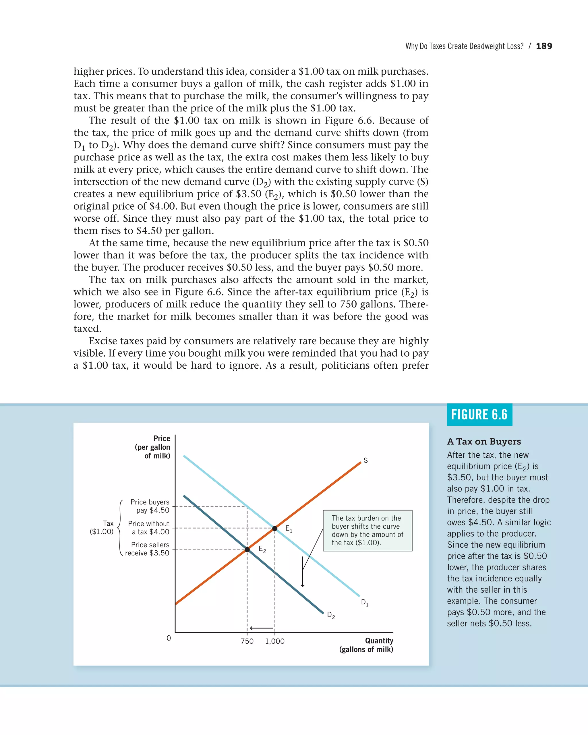
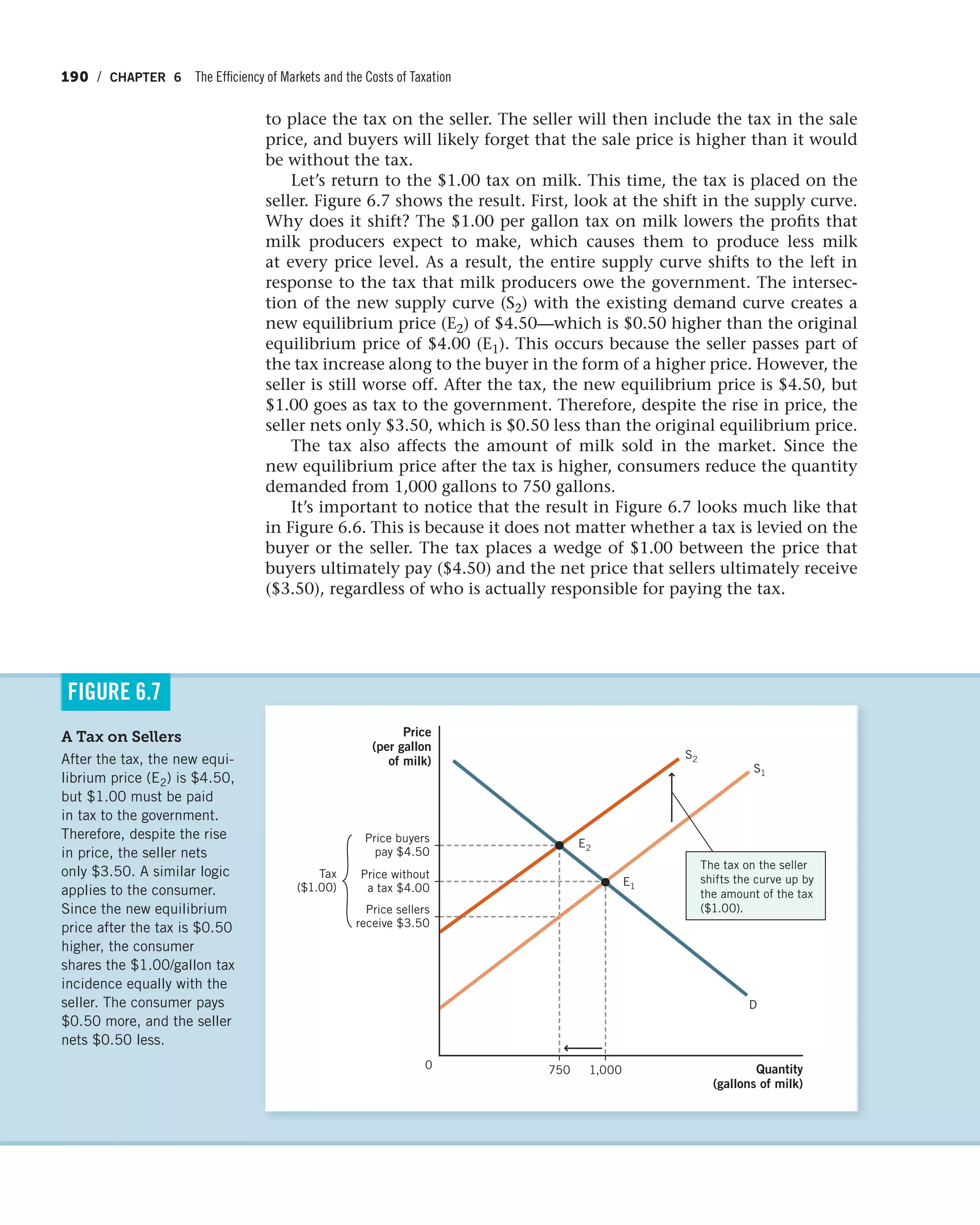
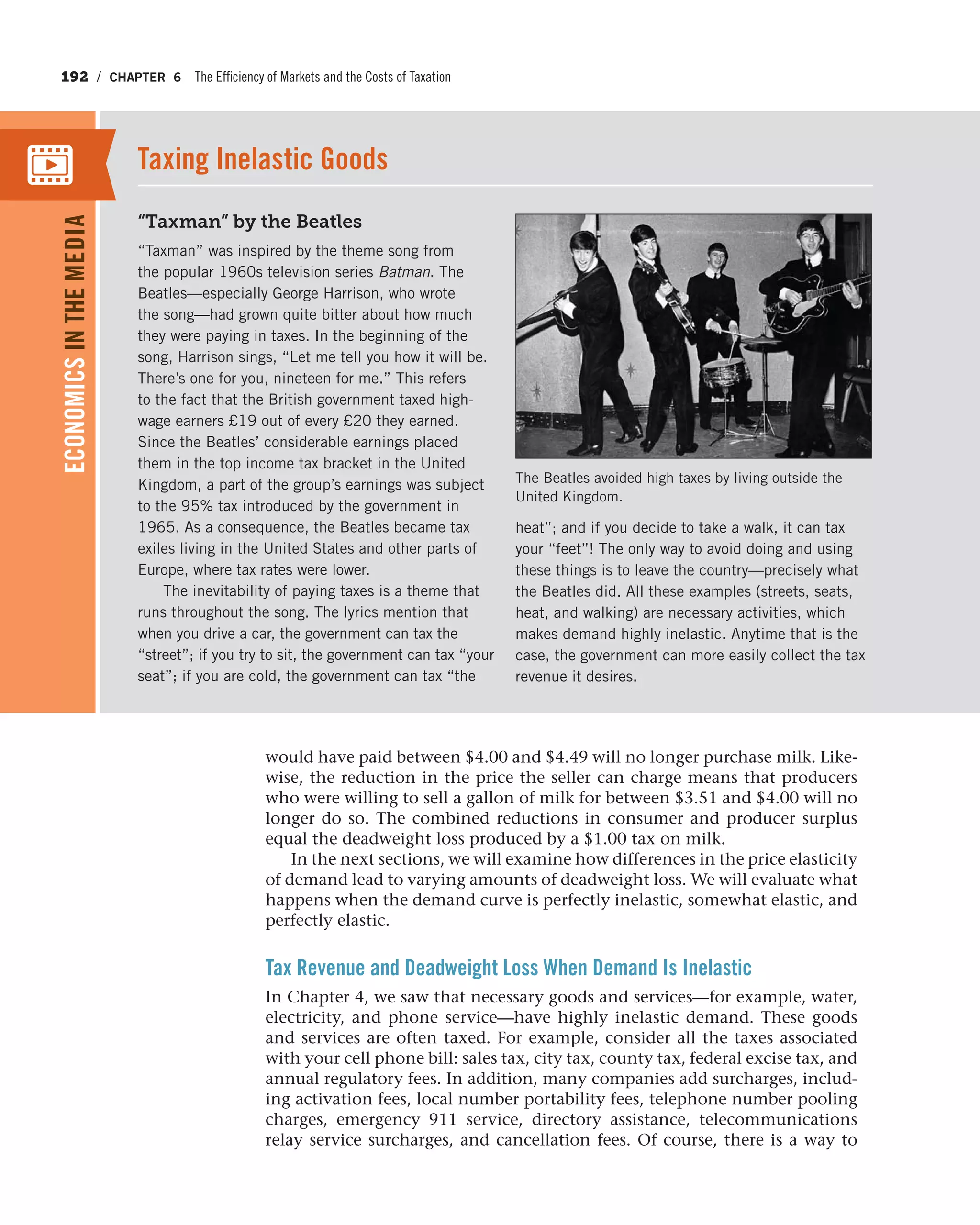
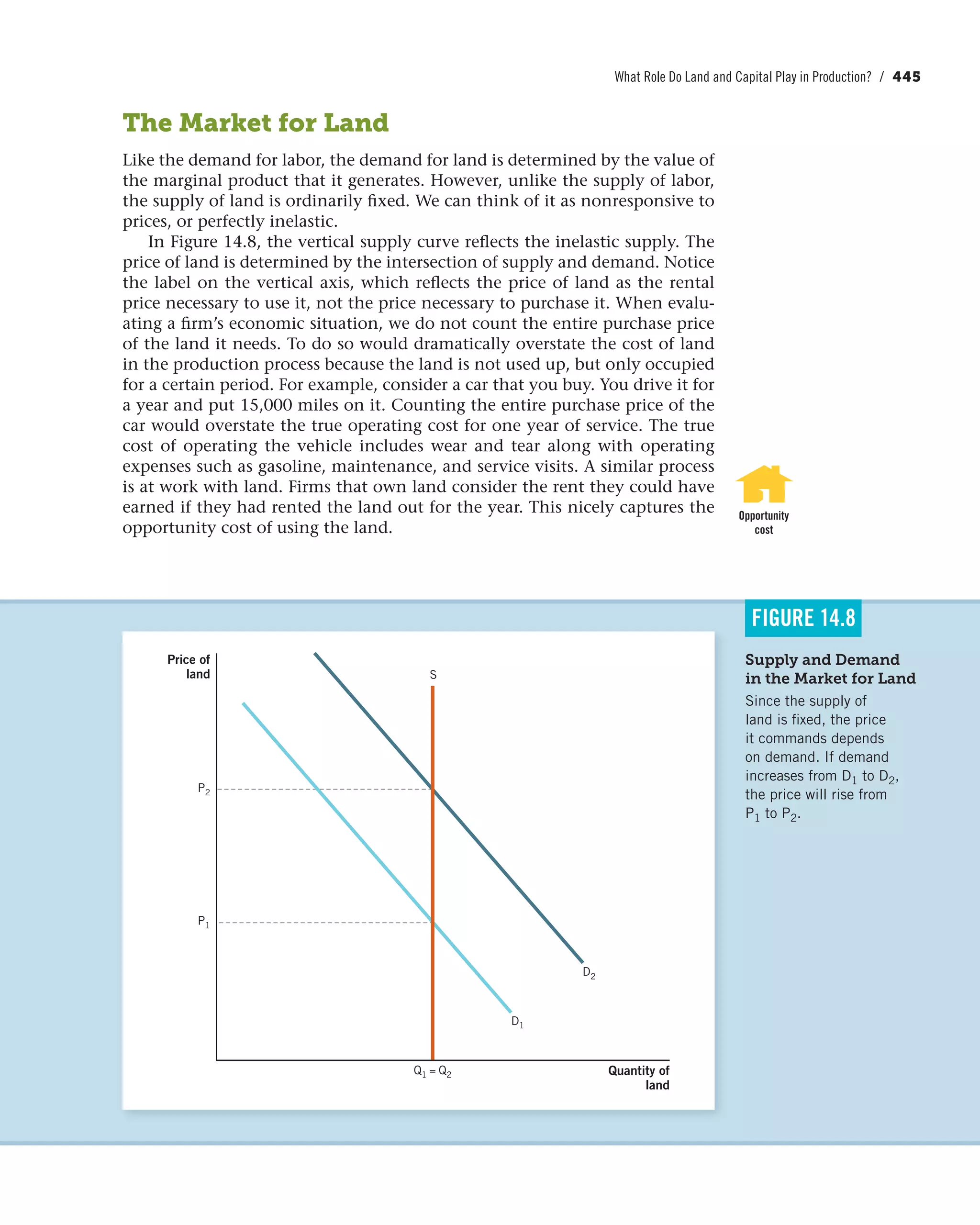
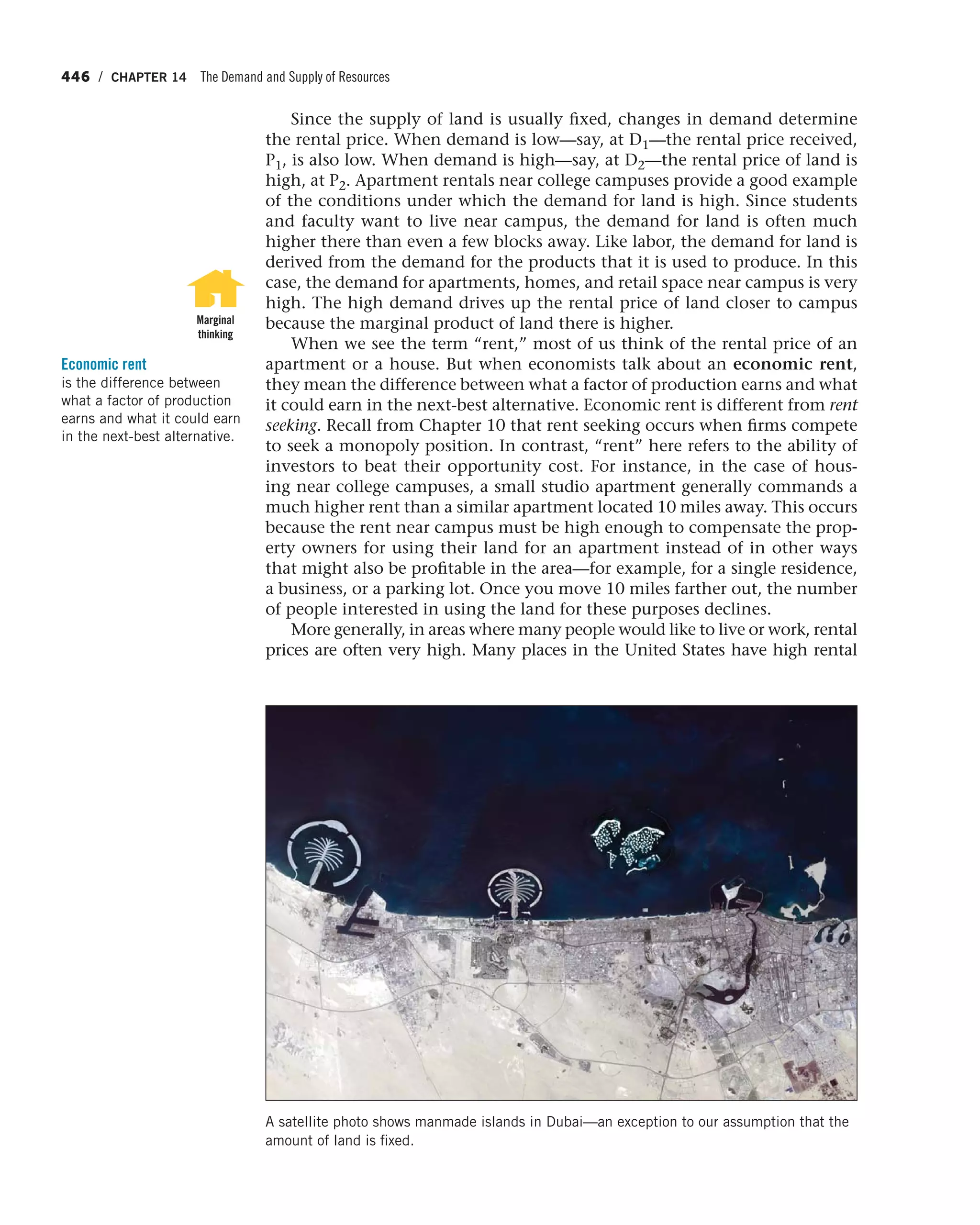
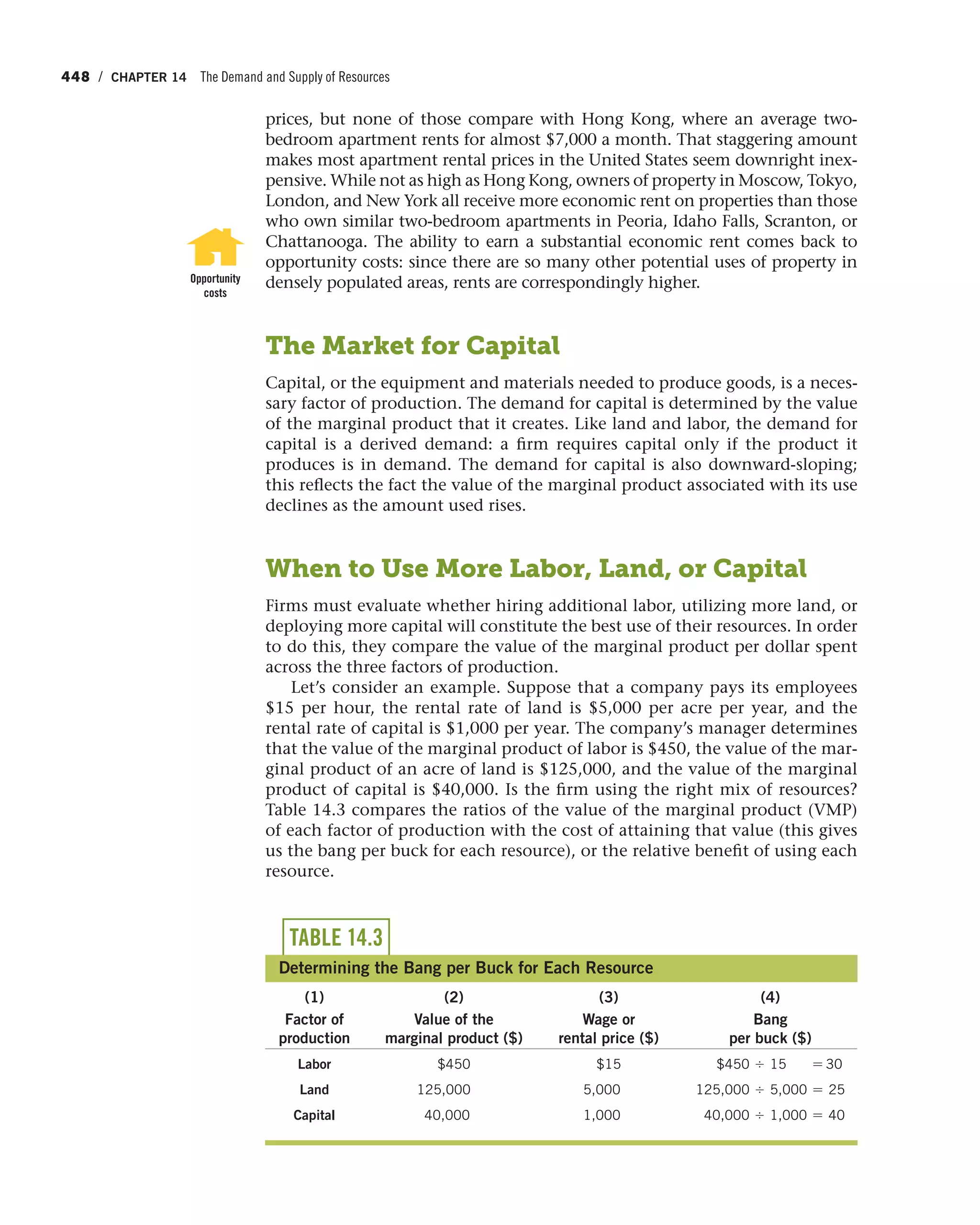
This document provides an overview and table of contents for the textbook "Principles of Economics" by Dirk Mateer and Lee Coppock. It was published by W.W. Norton & Company, which has been independently owned by its employees since the 1950s. The textbook covers microeconomic and macroeconomic concepts across 33 chapters organized into 10 parts. It includes examples, graphs, and discussions of economic principles and how they apply to real-world situations and current events. The authors provide brief biographies dedicating the book to their fathers for encouraging them in teaching economics.


![Reinforcers
Practice What You Know boxes are in-
chapter exercises that allow students
to self-assess while reading and provide
a bit more hand-holding than usual.
While other books have in-chapter ques-
tions, no other book consistently frames
these exercises within real-world situa-
tions that students relate to.
Income Elasticity
Question: A college student eats ramen noodles twice
a week and earns $300/week working part-time. After
graduating, the student earns $1,000/week and eats
ramen noodles every other week. What is the student’s
income elasticity?
Answer: The income elasticity of demand using the midpoint method is
EI =
(Q2 - Q1) , [(Q1 + Q2) , 2]
(I2 - I1) , [(I1 + I2) , 2]
Plugging in yields
EI =
(0.5 - 2.0) , [(2.0 + 0.5) , 2]
($1000 - $300) , [($300 + $1000) , 2]
Simplifying yields
EI =
-1.5 , 1.25
$700 , $650
Therefore, EI = -1.1.
The income elasticity of demand is positive for normal goods and negative
for inferior goods. Therefore, the negative coefficient indicates that ramen noo-
dles are an inferior good over the range of income—in this example, between
$300 and $1,000. This result should confirm your intuition. The higher post-
graduation income enables the student to substitute away from ramen noodles
and toward other meals that provide more nourishment and enjoyment.
PRACTICE WHAT YOU KNOW
Yummy, or all you can afford?
d
2
2
-
EI
ma
e
h
st
v
AAnswer The income elasticity ofAnswer: The income elasticity of
EI =
(Q2
(I
Plugging in yields
EI =
(0.5
($1000 -
Simplifying yields
E
Therefore, EI = -1.1.
The income elasticity of dem
for inferior goods. Therefore, the
dles are an inferior good over the
$300 and $1,000. This result sh
graduation income enables the s
and toward other meals that prov
Suppose that a local pizza place likes to run a “late-night special” after
11 p.m. The owners have contacted you for some advice. One of the owners
tells you, “We want to increase the demand for our pizza.” He proposes two
marketing ideas to accomplish this:
1. Reduce the price of large pizzas.
2. Reduce the price of a complementary good—for example, offer two half-
priced bottles or cans of soda with every large pizza ordered.
Question: What will you recommend?
Answer: First, consider why “late-night specials” exist in the first place. Since
most people prefer to eat dinner early in the evening, the store has to encour-
age late-night patrons to buy pizzas by stimulating demand. “Specials” of all
sorts are used during periods of low demand when regular prices would leave
the establishment largely empty.
Next, look at what the question asks. The owners want to know which
option would “increase demand” more. The question is very specific; it is
looking for something that will increase (or shift) demand.
PRACTICE WHAT YOU KNOW
Cheap pizza or . . . . . . cheap drinks?
D1
Price
(dollars
per pizza)
Quantity (pizza)
A reduction in the
price of pizza causes
a movement along the
demand curve.
Shift or Slide?
(CONTINUED)
Preface / xxxvii](https://image.slidesharecdn.com/principlesofeconomics-150728171823-lva1-app6892/75/Principles-of-economics-39-2048.jpg)


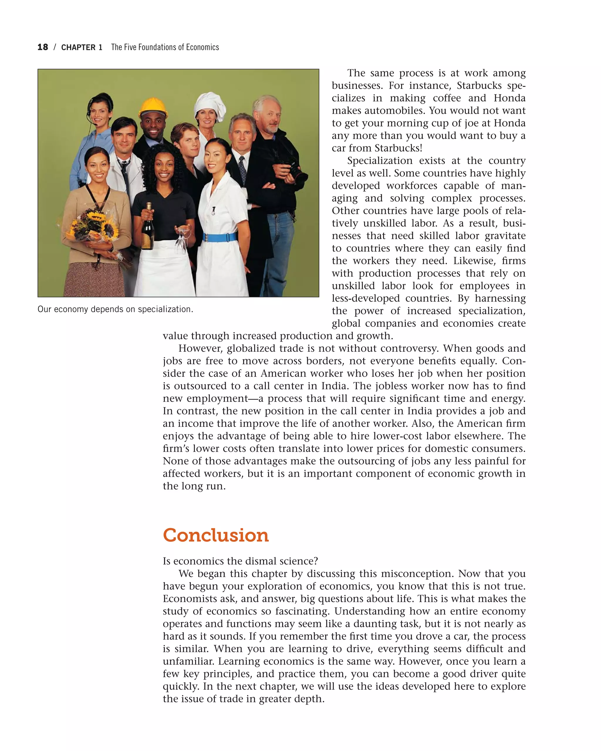
![8 / CHAPTER 1 The Five Foundations of Economics
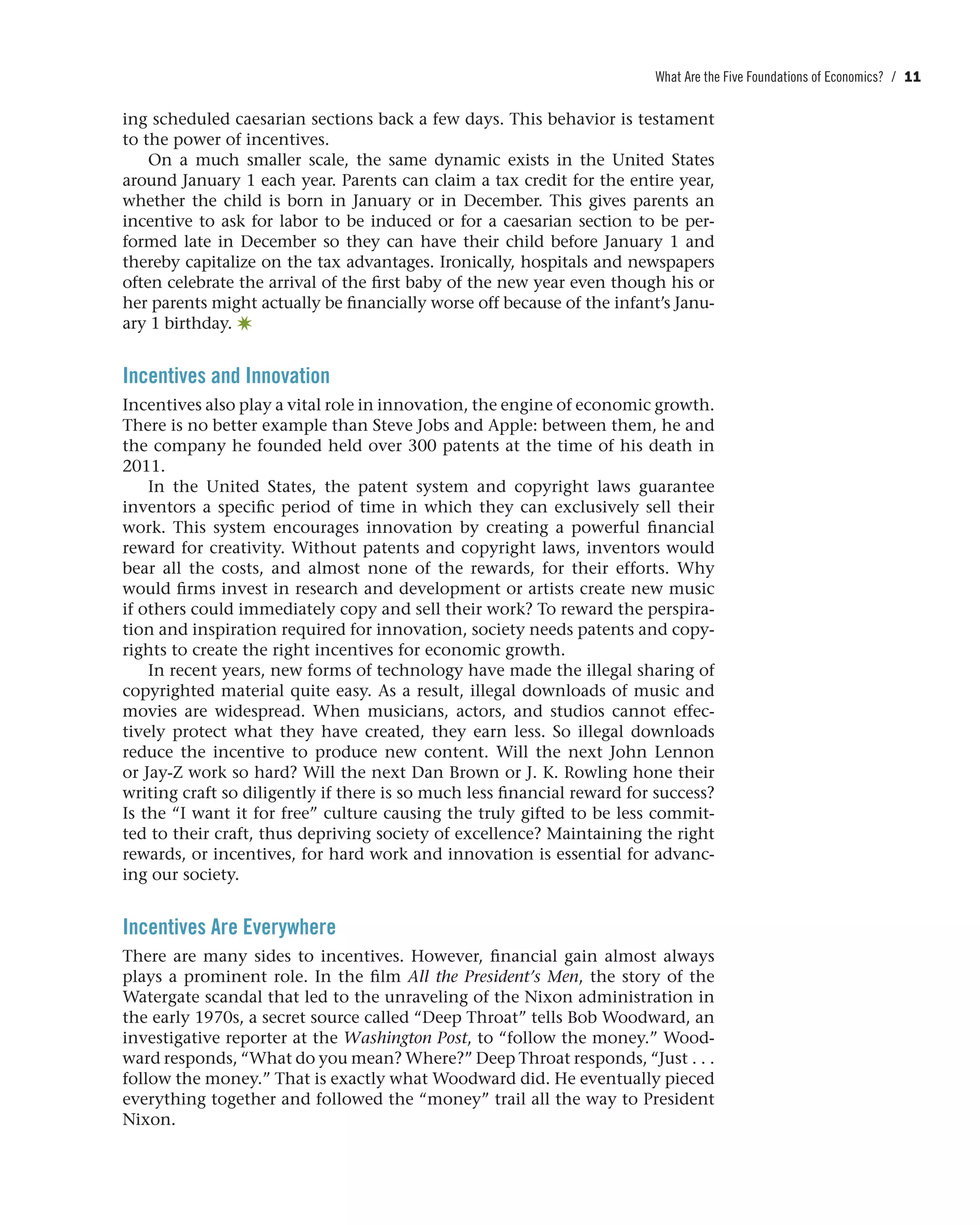
Positive and Negative Incentives
Positive incentives are those that encourage action. For example, end-of-the-
year bonuses motivate employees to work hard throughout the year, higher oil
prices cause suppliers to extract more oil, and tax rebates encourage citizens to
spend more money. Negative incentives also encourage action. For instance,
the fear of receiving a speeding ticket keeps motorists from driving too fast, and
the dread of a trip to the dentist motivates people to brush their teeth regularly.
In each case, a potential negative consequence spurs individuals to action.
Microeconomics and Macroeconomics:
The Big Picture
Identify whether each of the following state-
ments identifies a microeconomic or a macro-
economic issue.
The national savings rate is less than 2% of
disposable income.
Answer: The national savings rate is a
statistic based on the average amount
each household saves as a percentage of
income. As such, this is a broad measure
of savings and something that describes a
macroeconomic issue.
Jim was laid off from his last job and is currently
unemployed.
Answer: Jim’s personal financial circumstances constitute a microeconomic
issue.
Apple decides to open up 100 new stores.
Answer: Even though Apple is a very large corporation and 100 new stores will
create many new jobs, Apple’s decision is a microeconomic issue because
the basis for its decision is best understood as part of the firm’s competitive
strategy.
The government passes a jobs bill designed to stabilize the economy during a recession.
Answer: You might be tempted to ask how many jobs are created before
deciding, but that is not relevant to this question. The key part of the
statement refers to “stabiliz[ing] the economy during a recession.” This is an
example of a fiscal policy, in which the government takes an active role in
managing the economy. Therefore, it is a macroeconomic issue.
PRACTICE WHAT YOU KNOW
This mosaic of the flag illustrates the difference between micro and
macro.](https://image.slidesharecdn.com/principlesofeconomics-150728171823-lva1-app6892/75/Principles-of-economics-62-2048.jpg)


![116 / CHAPTER 4 Elasticity
The Midpoint Method
The calculation above was simple because we looked at the change in price
and the change in the quantity demanded from only one direction—that is,
from a high price to a lower price. However, the complete—and proper—way
to calculate elasticity is from both directions. Consider the following demand
schedule (it doesn’t matter what the product is):
Price Quantity demanded
$12 20
$ 6 30
Let’s calculate the elasticity of demand. If the price drops from $12 to
$6—a drop of 50%—the quantity demanded increases from 20 to 30—a rise
of 50%. Plugging the percentage changes into ED yields
Price Elasticity of Demand = ED =
50%
-50%
= -1.0
But if the price rises from $6 to $12—an increase of 100%—the quantity
demanded falls from 30 to 20, or decreases by 33%. Plugging the percentage
changes into ED yields
Price Elasticity of Demand = ED =
-33%
100%
= -0.33
This result occurs because percentage changes are usually calculated by using
the initial value as the base, or reference point. In this example, we worked the
problem two ways: by using $12 as the starting point and dropping the price
to $6, and by using $6 as the starting point and increasing the price to $12.
Even though we are measuring elasticity over the same range of values, the
percentage changes are different.
To avoid this problem, economists use the midpoint method, which gives
the same answer for the elasticity no matter what point you begin with. Equa-
tion 4.2 uses the midpoint method to express the price elasticity of demand.
While this equation looks more complicated than Equation 4.1, it is not. The
midpoint method merely specifies how to plug in the initial and ending val-
ues for price and the quantity to determine the percentage changes. Q1 and
P1 are the initial values, and Q2 and P2 are the ending values.
ED =
change in Q , average value of Q
change in P , average value of P
=
(Q2 - Q1) , [(Q1 + Q2) , 2]
(P2 - P1) , [(P1 + P2) , 2]
The change in the quantity demanded, (Q2 - Q1), and the change in price,
(P2 - P1), are each divided by the average of the initial and ending values, or
[(Q1 + Q2) , 2] and [(P1 + P2) , 2], to provide a way of calculating elasticity.
(Equation 4.2)](https://image.slidesharecdn.com/principlesofeconomics-150728171823-lva1-app6892/75/Principles-of-economics-170-2048.jpg)
![What Is the Price Elasticity of Demand, and What Are Its Determinants? / 117
The midpoint method is the preferred method for solving elasticity prob-
lems. To see why this is the case, let’s return to our pizza demand example.
If the price rises from $6 to $12, the quantity demanded falls from 30
to 20. Here the initial values are P1 = $6 and Q1 = 30. The ending values are
P2 = $12 and Q2 = 20. Using the midpoint method:
ED =
(20 - 30) , [(30 + 20) , 2]
($12 - $6) , [($12 + $6) , 2]
=
-10 , 25
$6 , $9
= -0.58
If the price falls from $12 to $6, quantity rises from 20 to 30. This time, the
initial values are P1 = $12 and Q1 = 20. The ending values are P2 = $6 and
Q2 = 30. Using the midpoint method:
ED =
(30 - 20) , [(20 + 30) , 2]
($6 - $12) , [($6 + $12) , 2]
=
10 , 25
-$6 , $9
= -0.58
When we calculated the price elasticity of demand from $6 to $12 using $6
as the initial point, ED = -0.33. Moving in the opposite direction, from $12
to $6, made $12 the initial reference point and ED = -1.0. The midpoint
method shown above splits the difference and uses $9 and 25 pizzas as
the midpoints. This approach makes the calculation of the elasticity coeffi-
cient the same, -0.58, no matter what direction the price moves. Therefore,
economists use the midpoint method to standardize the results. So, using
the midpoint method, we arrived at an elasticity coefficient of -0.58, which
is between 0 and -1. What does that mean? In this case, the percentage
change in the quantity demanded is less than the percentage change in
the price. Whenever the percentage change in the quantity demanded is
smaller than the percentage change in price, we say that demand is inelas-
tic. In other words, the price drop does not make a big difference in how
much pizza consumers purchased from the pizza shop. When the elasticity
coefficient is less than -1, the opposite is true, and we say that demand is
elastic.
Graphing the Price Elasticity of Demand
Visualizing elasticity graphically helps us understand the relationship
between elastic and inelastic demand. Figure 4.1 shows elasticity graph-
ically. As demand becomes increasingly elastic, or responsive to price
changes, the demand curve flattens.
Figure 4.1a depicts the price elasticity for pet care. Many pet own-
ers report that they would pay any amount of money to help their sick
or injured pet get better. (Of course, pet care is not perfectly inelastic,
because there is certainly a price beyond which some pet owners would
not or could not pay; but for illustrative purposes, let’s say that pet care
is perfectly elastic.) For these pet owners, the demand curve is a vertical
line. If you look along the Quantity axis, you will see that the quantity
of pet care demanded (QD) remains constant no matter what it costs. At
For many pet owners, the demand
for veterinary care is perfectly
inelastic.](https://image.slidesharecdn.com/principlesofeconomics-150728171823-lva1-app6892/75/Principles-of-economics-171-2048.jpg)


![128 / CHAPTER 4 Elasticity
The Price Elasticity of Demand
In this section, there are two questions to give you practice computing the
price elasticity of demand. Before we do the math, ask yourself whether you
think the price elasticity of demand for either subs or the antibiotic amoxicillin
is elastic.
Question: A store manager decides to lower the price of a featured sandwich from $3
to $2, and she finds that sales during the week increase from 240 to 480 sandwiches.
Is demand elastic?
Answer: Consumers were flexible and bought significantly more sandwiches in
response to the price drop. Let’s calculate the price elasticity of demand (ED)
using Equation 4.2. Recall that
ED =
(Q2 - Q1) , [(Q1 + Q2) , 2]
(P2 - P1) , [(P1 + P2) , 2]
Plugging in the values from above yields
ED =
(480 - 240) , [(240 + 480) , 2]
($2 - $3) , [($2 + $3) , 2]
=
240 , 360
-$1 , $2.50
Therefore, ED = -1.67.
Whenever the price elasticity of demand is less than -1, demand is consid-
ered elastic: the percentage change in the quantity demanded is greater than
the percentage change in price. This outcome is exactly what the store man-
ager expected. But subs are just one option for a meal; there are many other
choices, such as salads, burgers, and chicken—all of which cost more than
the now-reduced sandwich. Therefore, we should not be surprised that there
is a relatively large percentage increase in sub purchases by price-conscious
customers.
Question: A local pharmacy manager decides to raise the price of a 50-pill prescription
of amoxicillin from $8 to $10. The pharmacy tracks the sales of amoxicillin over the next
month and finds that sales decline from 1,500 to 1,480 boxes. Is the price elasticity of
demand elastic?
Answer: First, let’s consider the potential substitutes for amoxicillin. To
be sure, it’s possible to substitute other drugs, but they might not be as
effective. Therefore, most patients prefer to use the drug prescribed by their
doctor. Also, in this case the cost of the drug is relatively small. Finally,
patients’ need for amoxicillin is a short-run consideration. They want the
medicine now so they will get better! All three factors would lead us to believe
that the demand for amoxicillin is relatively inelastic. Let’s find out if that
intuition is confirmed in the data.
PRACTICE WHAT YOU KNOW
Is the demand for amoxicillin
elastic or inelastic?
(CONTINUED)
Is the demand for a sub
elastic or inelastic?](https://image.slidesharecdn.com/principlesofeconomics-150728171823-lva1-app6892/75/Principles-of-economics-182-2048.jpg)
![How Do Changes in Income and the Prices of Other Goods Affect Elasticity? / 129
have income elasticities between 0 and 1. For example,
expenditures on items such as milk, clothing, electricity, and
gasoline are unavoidable, and consumers at any income level
must buy them no matter what. Although purchases of neces-
sities will increase as income rises, they do not rise as fast as
the increase in income does. Therefore, as income increases,
spending on necessities will expand at a slower rate than the
increase in income.
Rising income enables consumers to enjoy significantly
more luxuries. This produces an income elasticity of demand
greater than 1. For instance, a family of modest means may
travel almost exclusively by car. However, as the family’s income rises, they
can afford air travel. A relatively small jump in income can cause the family
to fly instead of drive.
In Chapter 3, we saw that inferior goods are those that people will choose
not to purchase when their income goes up. Inferior goods have a nega-
tive income elasticity, because as income expands, the demand for the good
declines. We see this in Table 4.4 with the example of macaroni and cheese,
an inexpensive meal. As a household’s income rises, it is able to afford health-
ier food and more variety in the meals it enjoys. Consequently, the number
of times that mac and cheese is served declines. The decline in consumption
indicates that mac and cheese is an inferior good, and this is reflected in the
negative sign of the income elasticity.
The price elasticity of demand using the midpoint method is
ED =
(Q2 - Q1) , [(Q1 + Q2) , 2]
(P2 - P1) , [(P1 + P2) , 2]
Plugging in the values from the example yields
ED =
(1480 - 1500) , [(1480 + 1500) , 2]
($10 - $8) , [($8 + $10) , 2]
Simplifying produces this:
ED =
-20 , 1490
$2 , $9
Therefore, ED = -0.06. Recall that an ED near zero indicates that the price
elasticity of demand is highly inelastic, which is what we suspected. The price
increase does not cause consumption to fall very much. If the store manager had
been hoping to bring in a little extra revenue from the sales of amoxicillin, his
plan was successful. Before the price increase, the business sold 1,500 units
at $8, so revenues were $12,000. After the price increase, sales decreased to
1,480 units, but the new price is $10, so revenues now are $14,800. Raising
the price of amoxicillin helped the pharmacy make an additional $2,800 in
revenue.
(CONTINUED)
Air travel is a luxury good.](https://image.slidesharecdn.com/principlesofeconomics-150728171823-lva1-app6892/75/Principles-of-economics-183-2048.jpg)

![How Do Changes in Income and the Prices of Other Goods Affect Elasticity? / 131
TABLE 4.5
Cross-Price Elasticity
Type of good EI coefficient Example
Substitutes EC 7 0 Pizza Hut and
Domino’s
No relationship EC = 0 A basketball and
bedroom slippers
Complements EC 6 0 Turkey and
gravy
delicious.” From this, we can construct a cross-price elastic-
ity example. Suppose that the price of a two-liter bottle of
Mr. Pibb falls from $1.49 to $1.29. In the week immediately
preceding the price drop, a local store sells 60 boxes of Red
Vines. After the price drop, sales of Red Vines increase to 80
boxes. Let’s calculate the cross-price elasticity of demand
for Red Vines when the price of Mr. Pibb falls from $1.49 to
$1.29.
The cross-price elasticity of demand using the midpoint
method is
EC =
(QRV2 - QRV1) , [(QRV1 + QRV2) , 2]
(PMP2 - PMP1) , [(PMP1 + PMP2) , 2]
Notice that there are now additional subscripts to denote that we are measur-
ing the percentage change in the quantity demanded of good RV (Red Vines)
in response to the percentage change in the price of good MP (Mr. Pibb).
Plugging in the values from the example yields
EC =
(80 - 60) , [(60 + 80) , 2]
($1.29 - $1.49) , [($1.49 + $1.29) , 2]
Simplifying produces
EC =
20 , 70
-$0.20 , $1.39
Solving for EC gives us a value of -1.01. Because the result is a negative value,
this confirms our intuition that two goods that go well together (“crazy deli-
cious”) are complements, since the decrease in the price of Mr. Pibb causes
consumers to buy more Red Vines.
Have you tried Mr. Pibb and Red Vines together?](https://image.slidesharecdn.com/principlesofeconomics-150728171823-lva1-app6892/75/Principles-of-economics-185-2048.jpg)

![134 / CHAPTER 4 Elasticity
Income Elasticity
Question: A college student eats ramen noodles twice
a week and earns $300/week working part-time. After
graduating, the student earns $1,000/week and eats
ramen noodles every other week. What is the student’s
income elasticity?
Answer: The income elasticity of demand using the midpoint method is
EI =
(Q2 - Q1) , [(Q1 + Q2) , 2]
(I2 - I1) , [(I1 + I2) , 2]
Plugging in yields
EI =
(0.5 - 2.0) , [(2.0 + 0.5) , 2]
($1000 - $300) , [($300 + $1000) , 2]
Simplifying yields
EI =
-1.5 , 1.25
$700 , $650
Therefore, EI = -1.1.
The income elasticity of demand is positive for normal goods and negative
for inferior goods. Therefore, the negative coefficient indicates that ramen noo-
dles are an inferior good over the range of income—in this example, between
$300 and $1,000. This result should confirm your intuition. The higher post-
graduation income enables the student to substitute away from ramen noodles
and toward other meals that provide more nourishment and enjoyment.
PRACTICE WHAT YOU KNOW
Yummy, or all you can afford?
What Is the Price Elasticity of Supply?
Sellers, like consumers, are sensitive to price changes. However, the determi-
nants of the price elasticity of supply are substantially different from the deter-
minants of the price elasticity of demand. The price elasticity of supply is a
measure of the responsiveness of the quantity supplied to a change in price.
In this section, we examine how much sellers respond to price changes.
For instance, if the market price of gasoline increases, how will oil companies
respond? The answer depends on the elasticity of supply. Oil must be refined
into gasoline. If it is difficult for oil companies to increase their output of
gasoline significantly, even if the price increases a lot, the quantity of gasoline
supplied will not increase much. In this case, we say that the price elasticity
of supply is inelastic, or unresponsive. However, if the price increase is small
The price elasticity of supply
is a measure of the respon-
siveness of the quantity
supplied to a change in
price.](https://image.slidesharecdn.com/principlesofeconomics-150728171823-lva1-app6892/75/Principles-of-economics-188-2048.jpg)


![138 / CHAPTER 4 Elasticity
PRACTICE WHAT YOU KNOW
The Price Elasticity of Supply
Question: Suppose that the price of a barrel of oil increases
from $60 to $100. The new output is 2 million barrels a day,
and the old output is 1.8 million barrels. What is the price
elasticity of supply?
Answer: The price elasticity of supply using the
midpoint method is
ED =
(Q2 - Q1) , [(Q1 + Q2) , 2]
(P2 - P1) , [(P1 + P2) , 2]
Plugging in the values from the example yields
ES =
(2.0M - 1.8M) , [(1.8M + 2.0M) , 2]
($100 - $60) , [($60 + $100) , 2]
Simplifying yields
ES =
0.2M , 1.9M
$40 , $80
Therefore, ES = 0.20.
Recall from our discussion of the law of supply that there is a direct
relationship between the price and the quantity supplied. Since ES in this case
is positive, we see that output rises as price rises. However, the magnitude
of the output increase is quite small—this is reflected in the coefficient 0.20.
Because oil companies cannot easily change their production process, they
have a limited ability to respond quickly to rising prices. That inability is
reflected in a coefficient that is relatively close to zero. A zero coefficient
would mean that suppliers could not change their output at all. Here suppliers
are able to respond, but only in a limited capacity.
Oil companies have us
over a barrel.
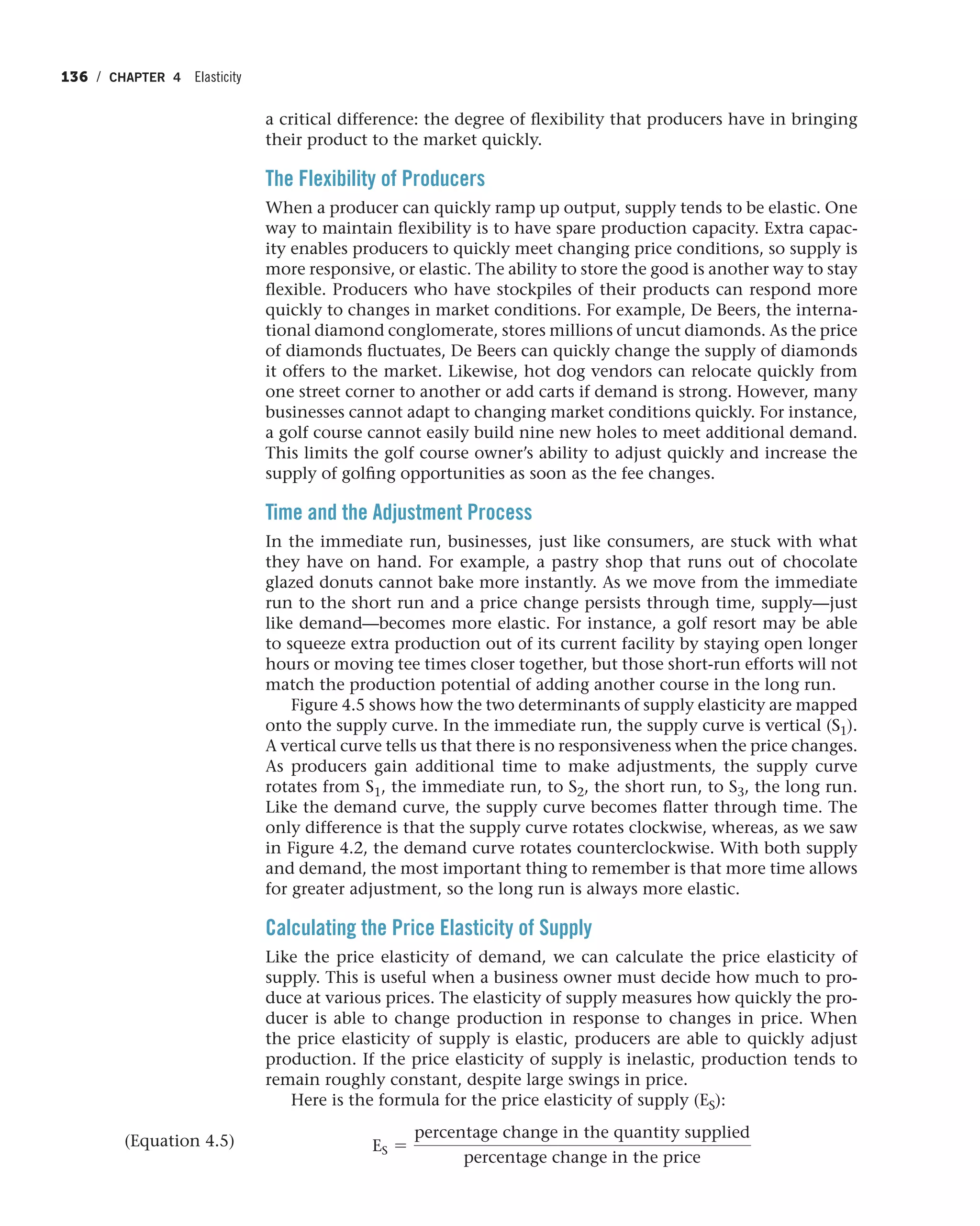
How Do the Price Elasticity of Demand
and Supply Relate to Each Other?
The interplay between the price elasticity of supply and the price elasticity of
demand allows us to explain more fully how the economy operates. With an
understanding of elasticity at our disposal, we can make a much richer and
deeper analysis of the world around us. For instance, suppose that we are con-
cerned about what will happen to the price of oil as economic development
spurs additional demand in China and India. An examination of the deter-
minants of the price elasticity of supply quickly confirms that oil producers](https://image.slidesharecdn.com/principlesofeconomics-150728171823-lva1-app6892/75/Principles-of-economics-192-2048.jpg)


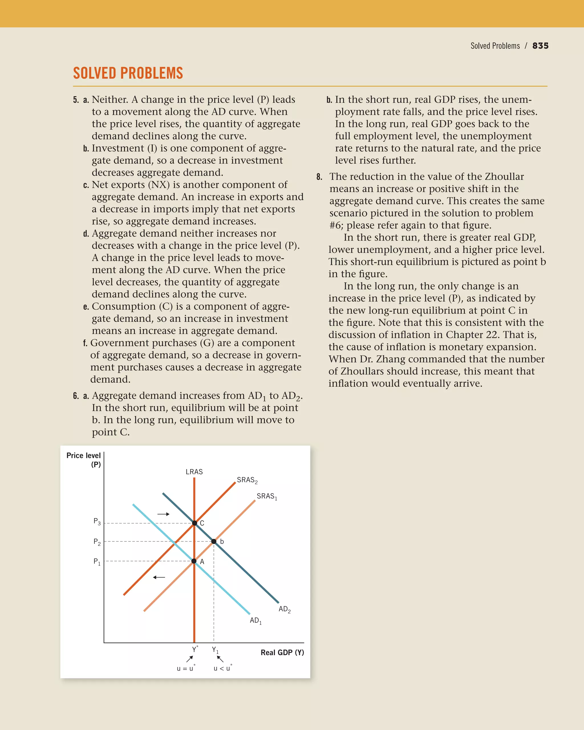
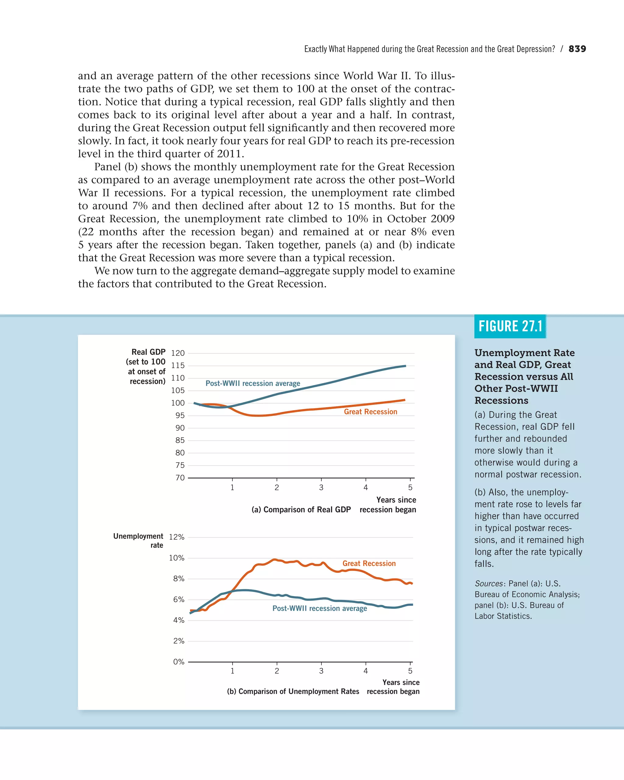
![Conclusion / 145
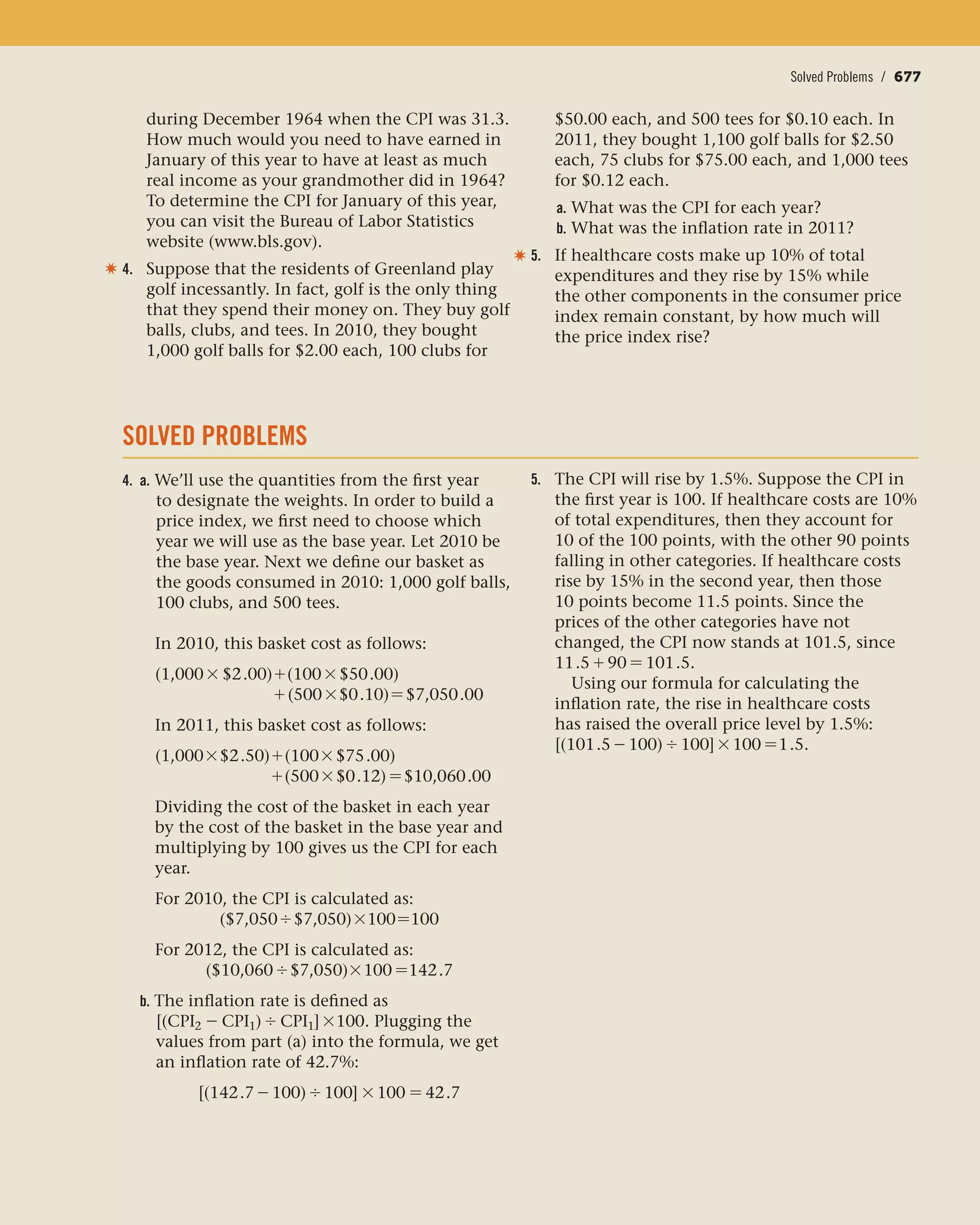
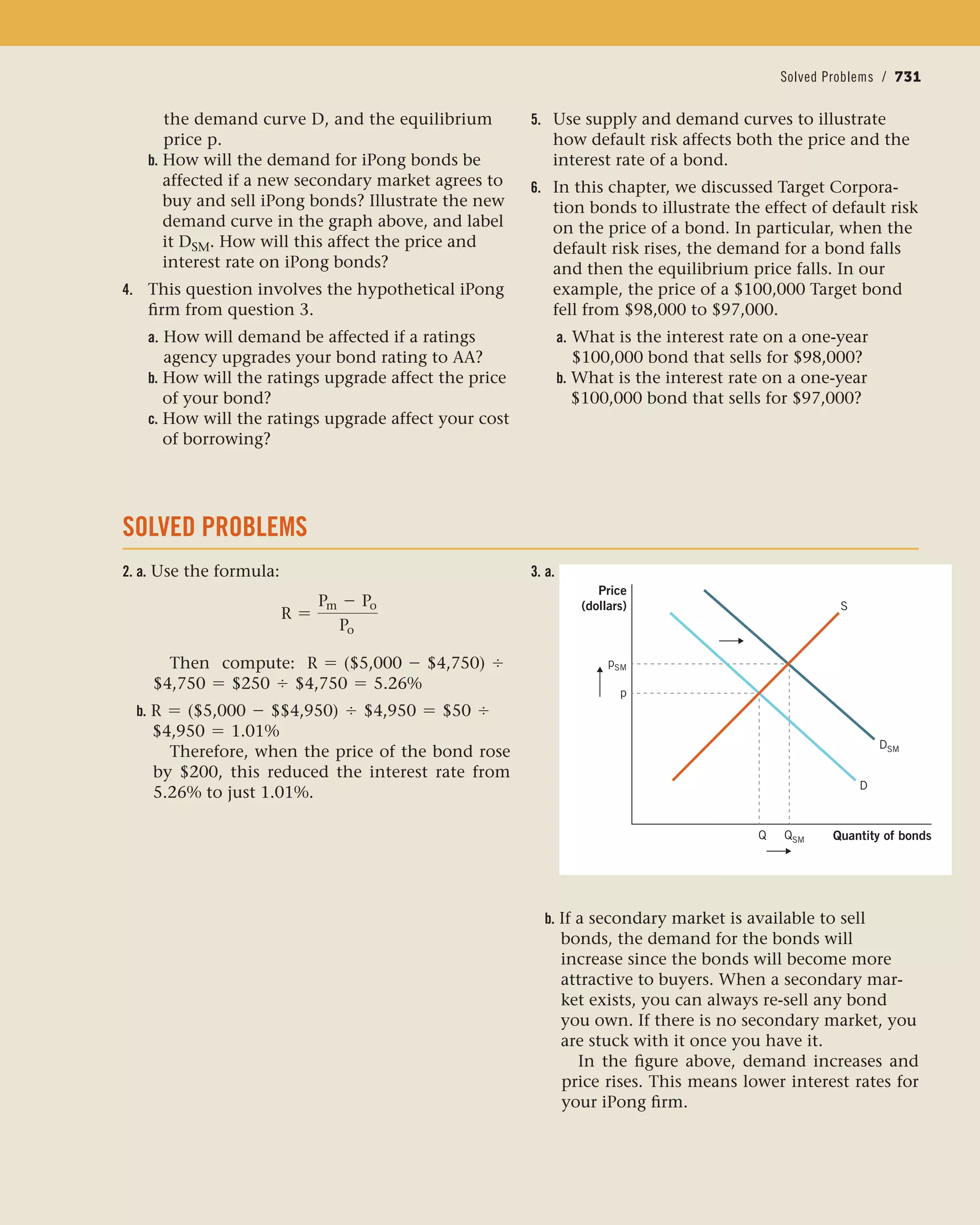
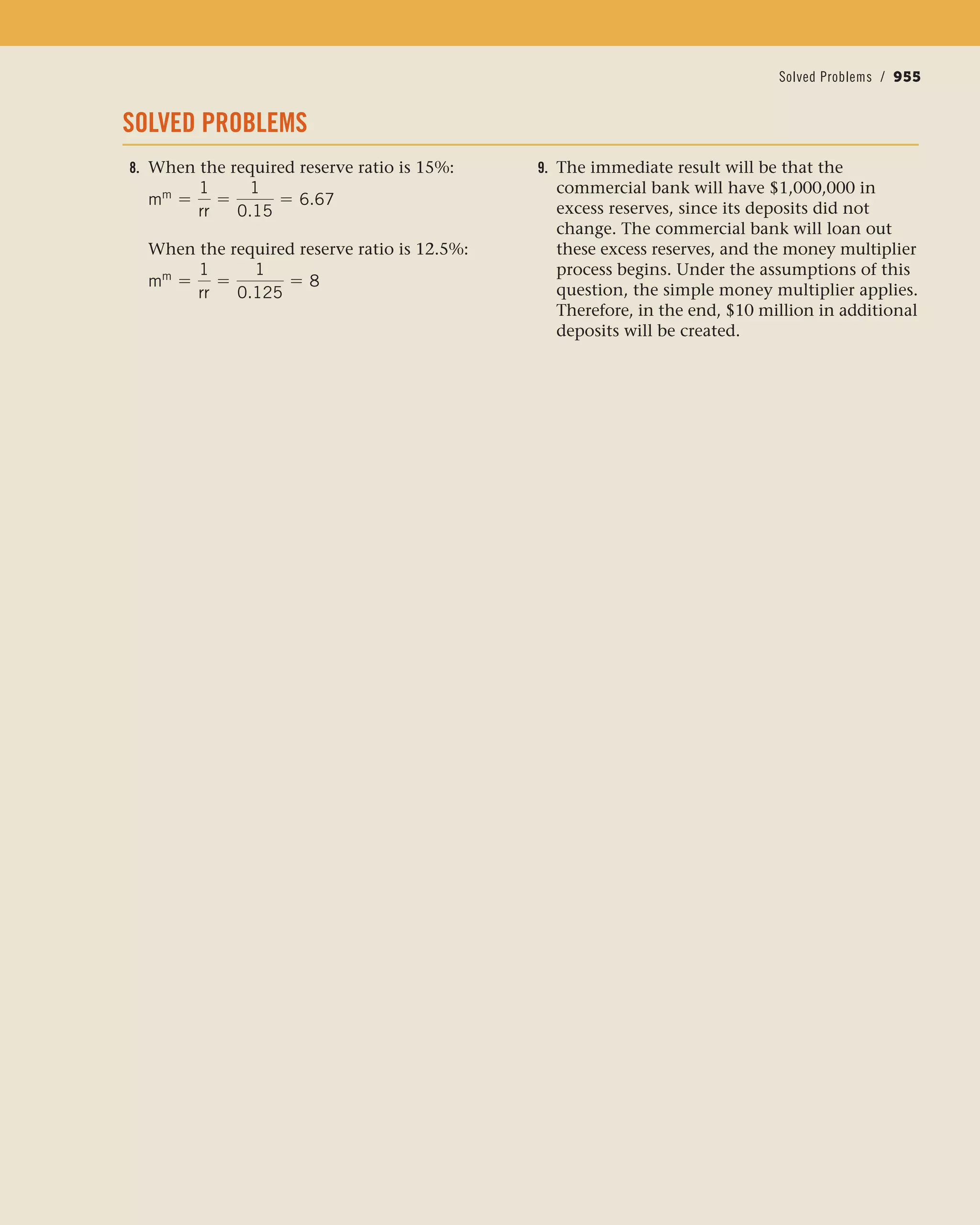
SOLVED PROBLEMS
1. To answer this question, we need to consider
the price elasticity of demand. The tax is
only on gray T-shirts. This means that T-shirt
customers who buy other colors can avoid the
tax entirely—which means that the demand
for gray T-shirts is relatively elastic. Since not
many gray T-shirts will be sold, the govern-
ment will generate a small increase in rev-
enues from the tax.
9. In this question a worker gets a 25% raise, so
we can use this information in the denomina-
tor when determining the income elasticity
of demand. We are not given the percentage
change for the meals out, so we need to plug
in how often the worker ate out before (once
a week) and the amount he eats out after the
raise (twice a week).
Plugging into EI gives us
EI =
(2 - 1) , [(1 + 2) , 2]
0.25
Simplifying yields
EI =
1 , 1.5
0.25
Therefore, EI = 2.67.
The income elasticity of demand for eating out
is positive for normal goods. Therefore, eating
out is a normal good. This result should con-
firm your intuition.
Let’s see what happens with frozen lasagna once
the worker gets the 25% raise. Now he cuts back
on the number of lasagna dinners from once a
week to once every other week.
Plugging into EI gives us
EI =
(0.5 - 1) , [(1 + 0.5) , 2]
0.25
Simplifying yields
EI =
-0.5 , 0.75
0.25
Therefore, EI = -2.67. The income elasticity of
demand for having frozen lasagna is negative.
Therefore, frozen lasagna is an inferior good.
This result should confirm your intuition.
Solved Problems / 145](https://image.slidesharecdn.com/principlesofeconomics-150728171823-lva1-app6892/75/Principles-of-economics-199-2048.jpg)


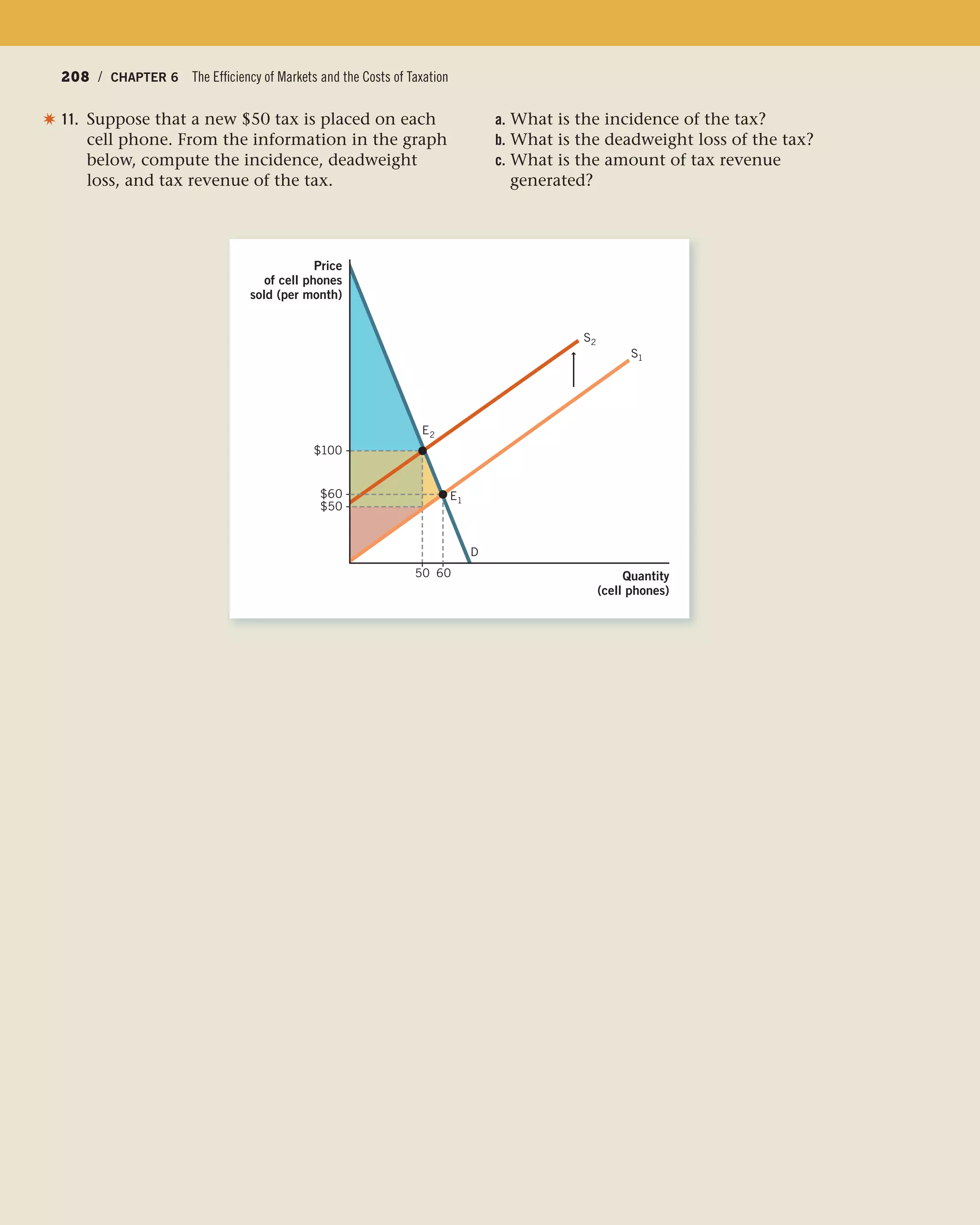
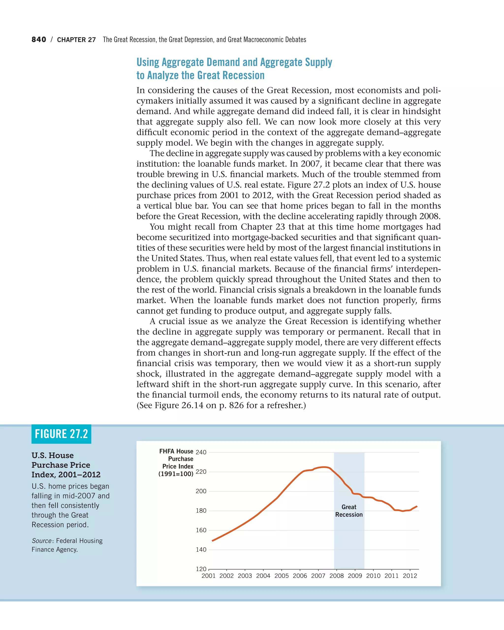
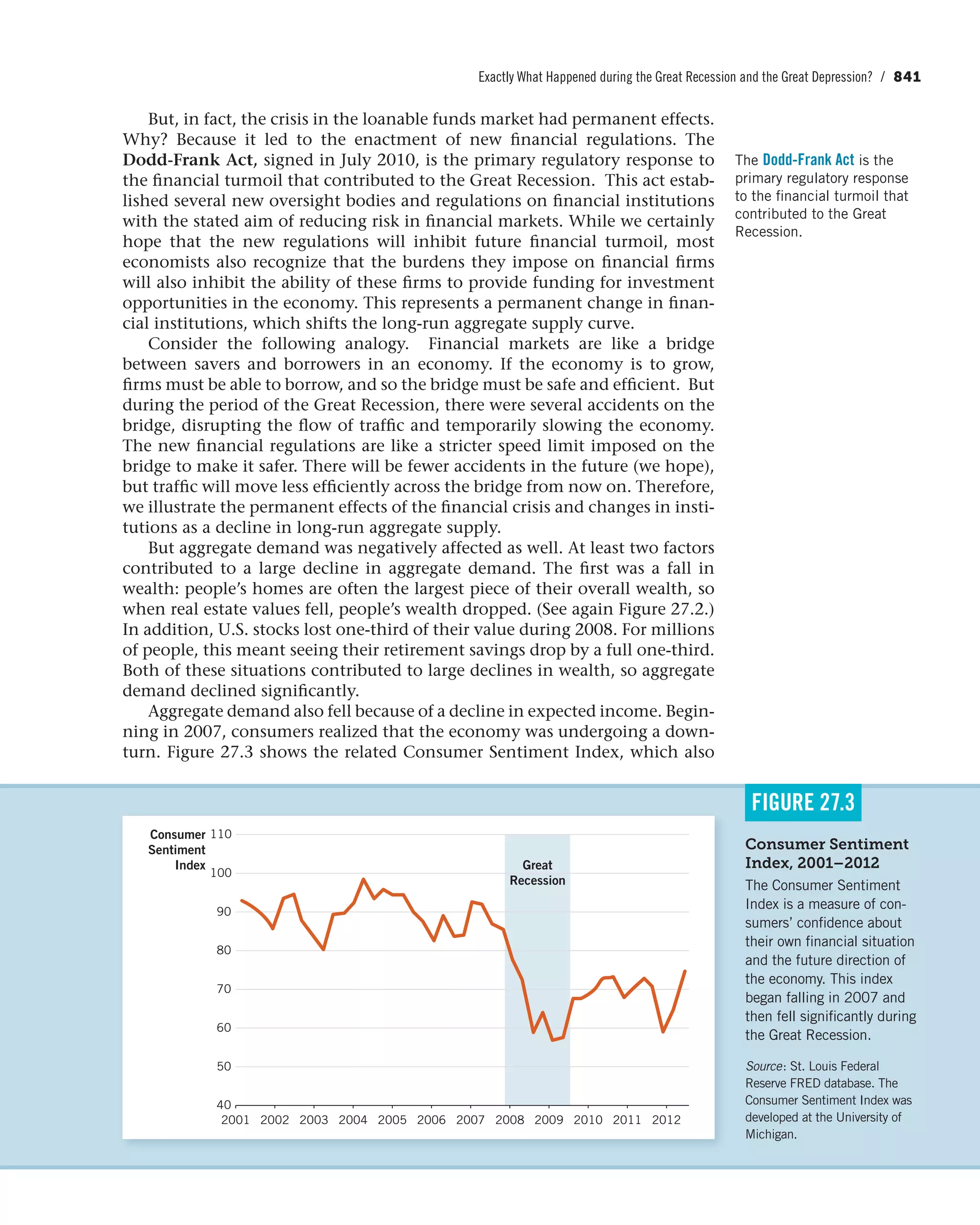
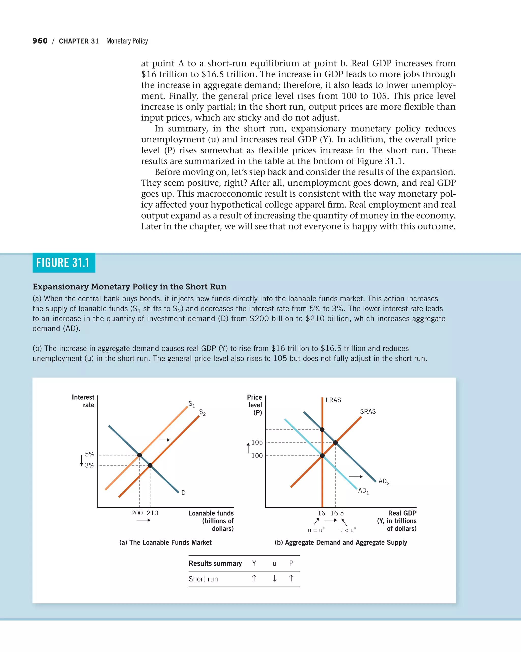
![Conclusion / 207
8. The cost of many electronic devices has fallen
appreciably since they were first introduced.
For instance, computers, cell phones, micro-
waves, and calculators not only provide more
functions but do so at a lower cost. Illustrate
the impact of lower production costs on the
supply curve. What happens to the size of the
consumer and producer surplus? If consumer
demand for cell phones is relatively elastic,
who is likely to benefit the most from the
lower production costs?
9. Suppose that the demand for a concert, QD,
is represented by the following equation,
where P is the price of concert tickets and
Q is the number of tickets sold:
QD = 2500 - 20P
The supply of tickets, QS, is represented by the
equation:
QS = -500 + 80P
a. Find the equilibrium price and quantity of
tickets sold. (Hint: Set QD = QS and solve
for the price, P, and then plug the result
back into either of the original equations to
find QE.)
b. Carefully graph your result in part a.
c. Calculate the consumer surplus at the equi-
librium price and quantity. (Hint: Since the
area of consumer surplus is a triangle, you
will need to use the formula for the area of
a triangle [1
2 * base * height] to solve the
problem.)
10. In this chapter, we have focused on the effect
of taxes on social welfare. However, govern-
ments also subsidize goods, or make them
cheaper to buy or sell. How would a $2,000
subsidy on the purchase of a new hybrid
vehicle impact the consumer surplus and
producer surplus in the hybrid market?
Use a supply and demand diagram to illustrate
your answer. Does the subsidy create dead-
weight loss?
Quantity
Price S2
C
D
F
B
A
E
D
S1
Amount
of the tax
Tax
Study Problems / 207](https://image.slidesharecdn.com/principlesofeconomics-150728171823-lva1-app6892/75/Principles-of-economics-261-2048.jpg)


![How Do Firms Maximize Profits? / 279
Once we know the profit-maximizing quantity, we can determine the average
cost of producing Q units. From Q, we move up along the dashed line until
it intersects with the ATC curve. From that point, we move horizontally until
we come to the y axis. This tells us the average cost of making 8 units. Since
the total cost in Table 9.3 is $70 when 8 driveways are plowed, dividing 70 by
8 gives us $8.75 for the average total cost. We can calculate Mr. Plow’s profit
rectangle from Figure 9.1 as follows:
Profit = (Price - ATC[along the dashed line at quantity Q]) * Q
This gives us (10-8.75) * 8 = $10, which is the profit we see in Table 9.3,
column 4, in red numbers. Since the MR is the price, and since the price is
higher than the average total cost, the firm makes the profit visually repre-
sented in the green rectangle.
The Firm in the Short Run
Deciding how much to produce in order to maximize profits is the goal of
every business. However, there are times when it is not possible to make a
profit. When revenue is insufficient to cover cost, the firm suffers a loss—at
which point it must decide whether to operate or temporarily shut down.
Successful businesses make this decision all the time. For example, retail
Profit Maximization
Mr. Plow uses the profit-
maximizing rule to locate
the point at which marginal
revenue equals marginal
cost, or MR = MC. This
determines the ideal out-
put level, Q. The firm takes
the price from the market;
this is shown as the
horizontal MR curve where
price = $10.00. Since
the price charged is higher
than the average total cost
curve along the dashed
line at quantity Q, the
firm makes the economic
profit shown in the green
rectangle.
FIGURE 9.1
P = $10.00
Q = 8
ATC = $8.75
Price
and Cost
Quantity
(driveways plowed)
MC
Profit
Maximum profit
occurs here, where
MR = MC
ATC
MR
A](https://image.slidesharecdn.com/principlesofeconomics-150728171823-lva1-app6892/75/Principles-of-economics-333-2048.jpg)


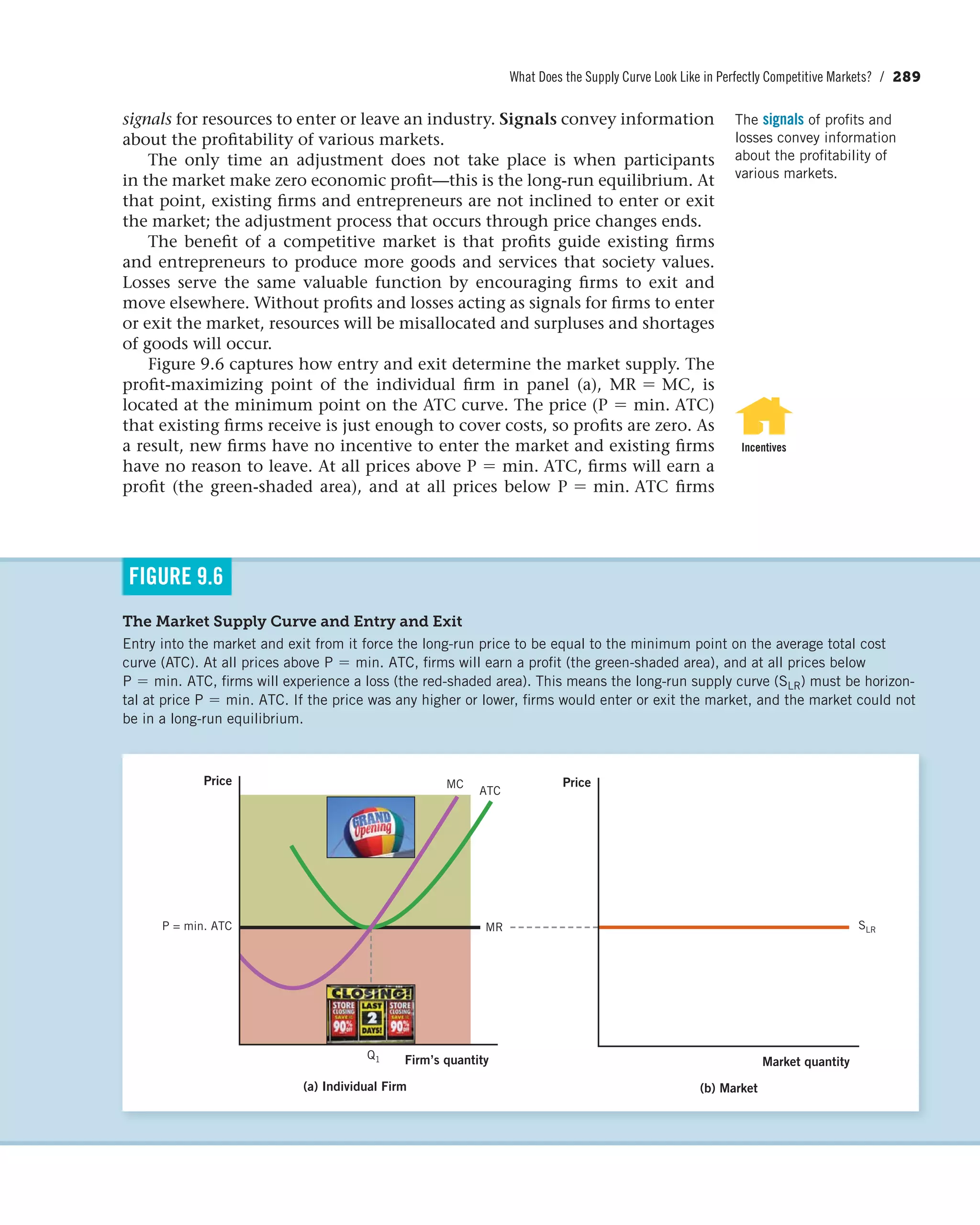

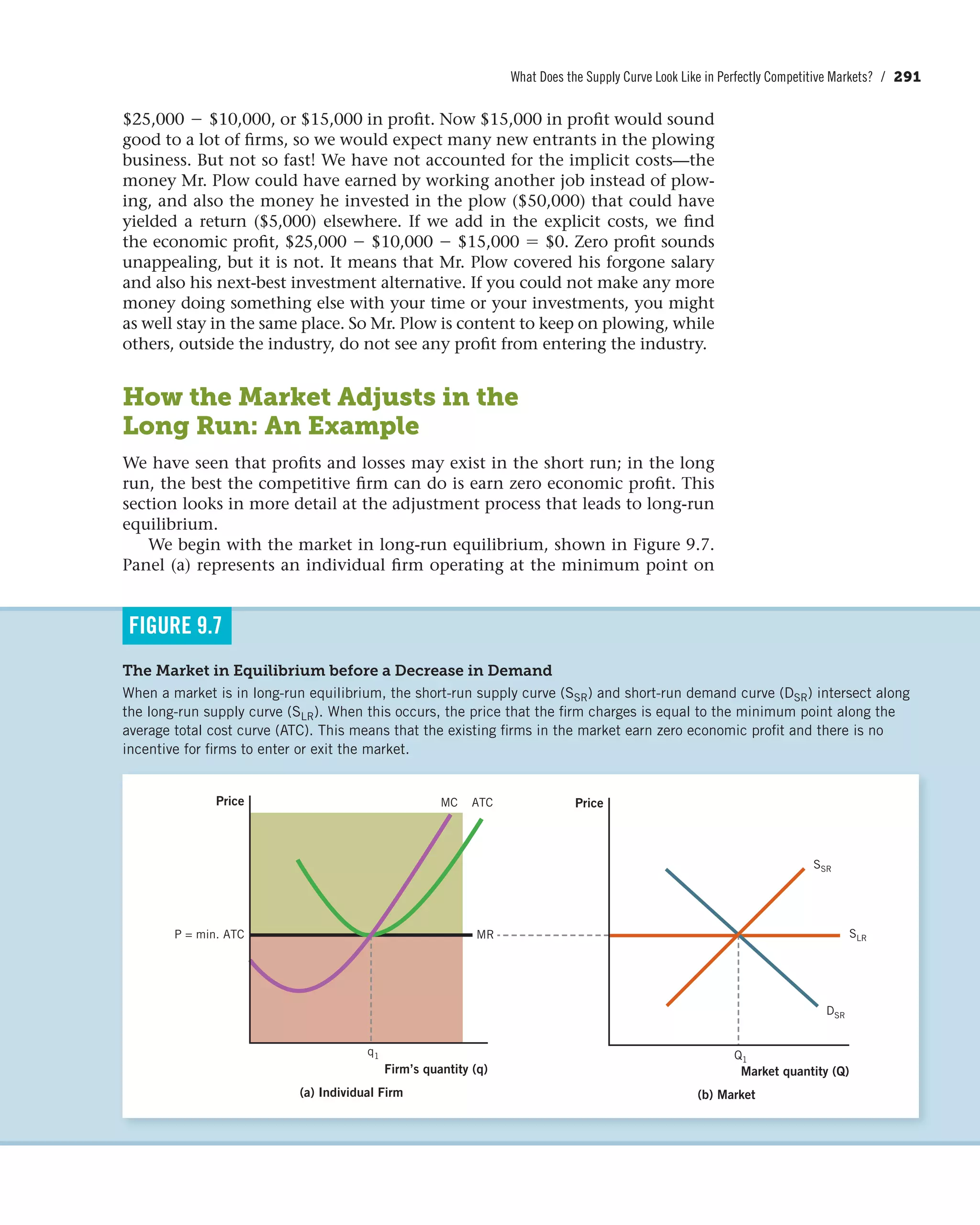
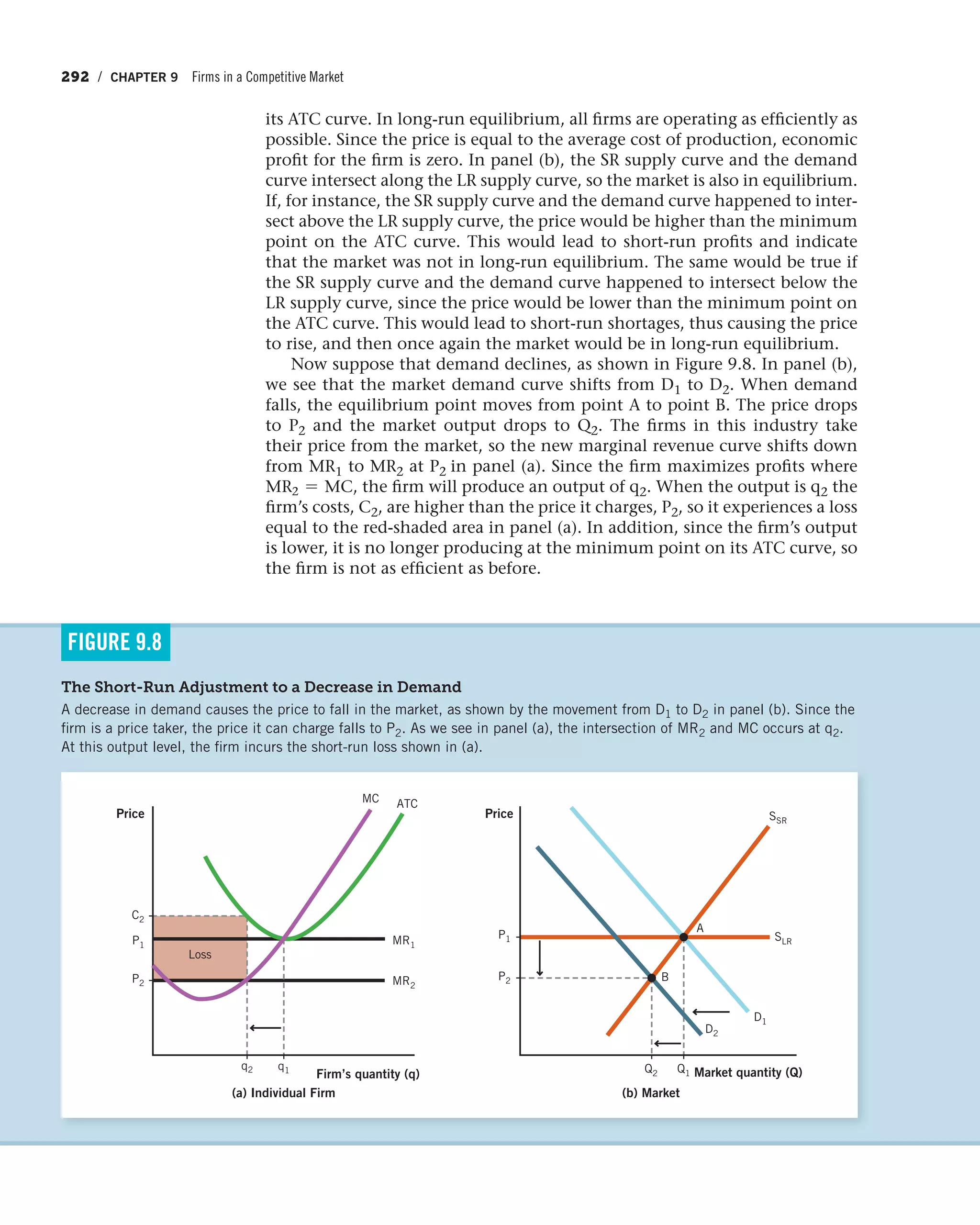
![What Does the Supply Curve Look Like in Perfectly Competitive Markets? / 293
I Love Lucy
I Love Lucy was the most watched television
comedy of the 1950s. The show featured two
couples who are best friends, the Ricardos and the
Mertzes, who find themselves in the most unlikely
situations.
One particular episode finds Ricky Ricardo disil-
lusioned with show business. After some conversa-
tion, Ricky and Fred Mertz decide to go into business
together and start a diner. Fred and Ethel Mertz have
the experience to run the diner, and Ricky plans to
use his name and star power to help get the word out
about the restaurant, which they name A Little Bit of
Cuba.
If you have seen any of the I Love Lucy series,
you already know that the business venture is des-
tined to fail. Sure enough, the Mertzes get tired of
doing all of the hard work—cooking and serving the
customers—while Ricky and Lucy Ricardo meet and
greet the guests. Things quickly deteriorate, and the
two couples decide to part ways. The only problem
is that they are both part owners, and neither can
afford to buy out the other. So they decide to split
the diner in half right down the middle!
The result is absurd and hilarious. On one side,
guests go to A Little Bit of Cuba. On the other side,
the Mertzes set up Big Hunk of America. Since both
restaurants use the same facilities and sell the same
food, the only way they can differentiate themselves
is by lowering their prices. This leads to a hamburger
price war to attract customers:
Ethel: “Three!”
Lucy: “Two!”
Ethel: “One-cent hamburgers.”
Fred: “Ethel, are you out of your mind?” [Even
in the 1950s, a penny was not enough
to cover the marginal cost of making a
hamburger.]
Ethel: “Well, I thought this could get ’em.”
Fred: “One-cent hamburgers?”
After the exchange, Lucy whispers in a
customer’s ear and gives him a dollar. He then
proceeds to Big Hunk of America and says,
“I’d like 100 hamburgers!”
Fred Mertz replies, “We’re all out of
hamburgers.”
How do the falling prices described here
affect the ability of the firms in this market to
make a profit?
The exchange is a useful way of visualizing how
perfectly competitive markets work. Competition forces
the price down, but the process of entry and exit takes
time and is messy. The Ricardos and Mertzes can’t
make a living selling one-cent hamburgers—one cent
is below their marginal cost—so one of the couples
will end up exiting. At that point, the remaining
couple would be able to charge more. If they end up
making a profit, that profit will encourage entrepre-
neurs to enter the business. As the supply of ham-
burgers expands, the price that can be charged will
be driven back down. Since we live in an economi-
cally dynamic world, prices are always moving toward
the long-run equilibrium.
Entry and Exit
ECONOMICSINTHEMEDIA](https://image.slidesharecdn.com/principlesofeconomics-150728171823-lva1-app6892/75/Principles-of-economics-347-2048.jpg)


![Negotiation Ch 1 Introduction [Sav Lecture]](https://cdn.slidesharecdn.com/ss_thumbnails/negotiationleweckich1introductionsavlecture-100301195744-phpapp01-thumbnail.jpg?width=640&height=640&fit=bounds)


