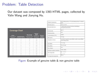
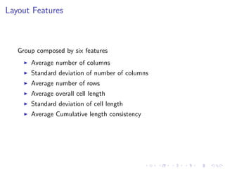
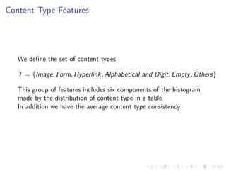
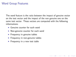
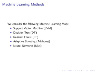
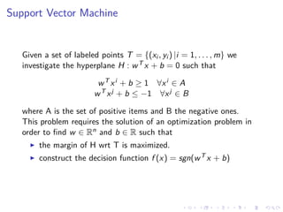
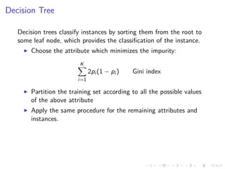
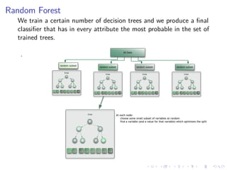
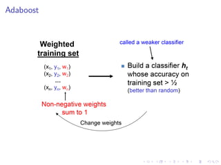
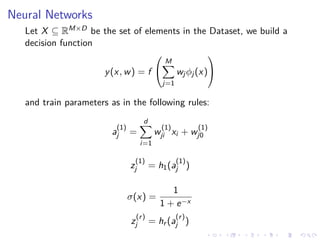
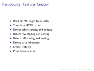
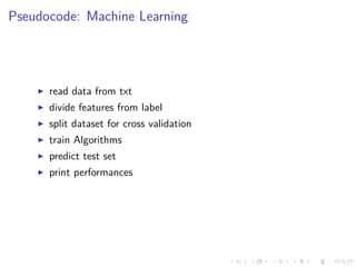
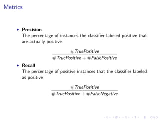
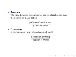
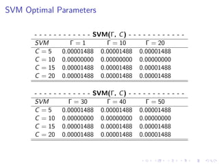
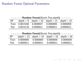
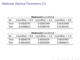
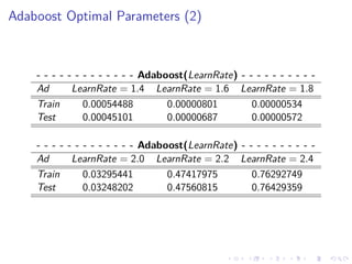
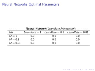
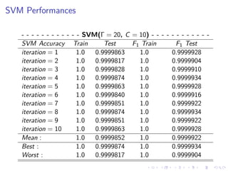
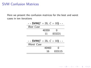
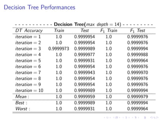
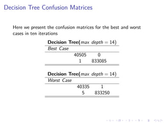
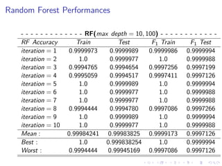
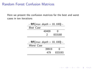
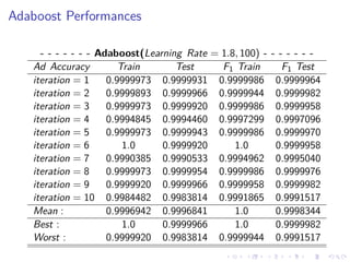
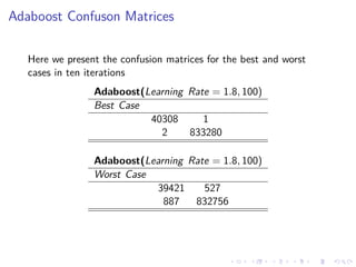
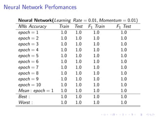
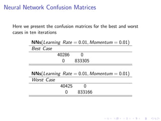
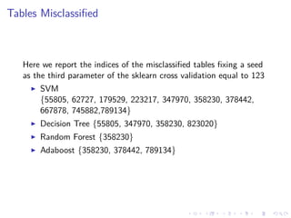
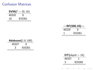
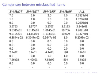
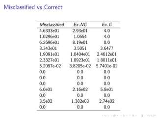
Web algorithm Project
Armenise Iolanda
Cataldi Alessandro
Filingeri Giuseppe
13 Ottobre 2016
Dott. Perehodko Eugeniya
Prof. Italiano Giuseppe
Problem: Table Detection
To recognize genuine and non genuine tables from HTML pages.
Genuine tables: entities where a structure is used to convey
the logical relations among the cells.
Non-genuine tables: entities where <TABLE> tags are used
to group contents into clusters for easy viewing only.
Problem: Table Detection
Our dataset was composed by 1393 HTML pages, collected by
Yalin Wang and Jianying Hu.
Figure: Example of genuine table & non genuine table
Features
We consider fourteen features divided in three different groups:
Layout Features
Content Type Features
Word Group Features
Layout Features
Group composed by six features
Average number of columns
Standard deviation of number of columns
Average number of rows
Average overall cell length
Standard deviation of cell length
Average Cumulative length consistency
Content Type Features
We define the set of content types
T = {Image, Form, Hyperlink, Alphabetical and Digit, Empty, Others}
This group of features includes six components of the histogram
made by the distribution of content type in a table
In addition we have the average content type consistency
Word Group Features
The word feature is the ratio between the impact of genuine vector
on the test vector and the impact of the non genuine one on the
same test vector. These vectors are computed with the following
informations:
Genuine counter for each word
Non-genuine counter for each word
Frequency in genuine tables
Frequency in non-genuine tables
Frequency in a new test table
Machine Learning Methods
We consider the following Machine Learning Model
Support Vector Machine (SVM)
Decision Tree (DT)
Random Forest (RF)
Adaptive Boosting (Adaboost)
Neural Networks (NNs)
Support Vector Machine
Given a set of labeled points T = {(xi , yi ) |i = 1, . . . , m} we
investigate the hyperplane H : wT x + b = 0 such that
wT xi + b ≥ 1 ∀xi ∈ A
wT xj + b ≤ −1 ∀xj ∈ B
where A is the set of positive items and B the negative ones.
This problem requires the solution of an optimization problem in
order to find w ∈ Rn and b ∈ R such that
the margin of H wrt T is maximized.
construct the decision function f (x) = sgn(wT x + b)
Decision Tree
Decision trees classify instances by sorting them from the root to
some leaf node, which provides the classification of the instance.
Choose the attribute which minimizes the impurity:
K
i=1
2pi (1 − pi ) Gini index
Partition the training set according to all the possible values
of the above attribute
Apply the same procedure for the remaining attributes and
instances.
Random Forest
We train a certain number of decision trees and we produce a final
classifier that has in every attribute the most probable in the set of
trained trees.
Adaboost
Neural Networks
Let X ⊆ RM×D be the set of elements in the Dataset, we build a
decision function
y(x, w) = f


M
j=1
wjφj(x)


and train parameters as in the following rules:
a
(1)
j =
d
i=1
w
(1)
ji xi + w
(1)
j0
z
(1)
j = h1(a
(1)
j )
σ(x) =
1
1 + e−x
z
(r)
j = hr (a
(r)
j )
Pseudocode: Features Creation
Read HTML pages from folder
Transform HTML to txt
Detect table starttag and endtag
Detect row startag and endtag
Detect cell startag and endtag
Detect data inbetween
Create features
Print features in txt
Pseudocode: Machine Learning
read data from txt
divide features from label
split dataset for cross validation
train Algorithms
predict test set
print performances
Metrics
Precision
The percentage of instances the classifier labeled positive that
are actually positive
#TruePositive
#TruePositive + #FalsePositive
Recall
The percentage of positive instances that the classifier labeled
as positive
#TruePositive
#TruePositive + #FalseNegative
Accuracy
The ratio between the number of correct classification over
the number of classification
#CorrectClassifications
#Classifications
F1-measure:
is the harmonic mean of precision and recall
2(Precision)(Recall)
Precision + Recall
SVM Optimal Parameters
- - - - - - - - - - - - SVM(Γ, C) - - - - - - - - - - - -
SVM Γ = 1 Γ = 10 Γ = 20
C = 5 0.00001488 0.00001488 0.00001488
C = 10 0.00000000 0.00000000 0.00000000
C = 15 0.00001488 0.00001488 0.00001488
C = 20 0.00001488 0.00001488 0.00001488
- - - - - - - - - - - - SVM(Γ, C) - - - - - - - - - - - -
SVM Γ = 30 Γ = 40 Γ = 50
C = 5 0.00001488 0.00001488 0.00001488
C = 10 0.00000000 0.00000000 0.00000000
C = 15 0.00001488 0.00001488 0.00001488
C = 20 0.00001488 0.00001488 0.00001488
Kernel plot
Figure: Example of Gaussian Kernel
Decision Tree Optimal Parameters
- - - - - - - - - - - - - Tree(depth) - - - - - - - - - - - - - -
DT depth = 3 depth = 5 depth = 8 depth = 12
Train 0.02978931 0.01694997 0.00527249 0.00109510
Test 0.02911431 0.01656725 0.00508934 0.00103824
- - - - - - - - - - - - - Tree(depth) - - - - - - - - - - - - - -
DT depth = 14 depth = 15 depth = 16 depth = 18
Train 0.00000267 0.00000000 0.00000000 0.00000000
Test 0.00000229 0.00000229 0.00000343 0.00000572
Random Forest Optimal Parameters
- - - - - - Random Forest(Numb.Tree,depth) - - - - - -
RF depth = 9 depth = 10 depth = 11 depth = 12
Train 0.0013168 0.0000027 0.0000000 0.0000000
Test 0.0013118 0.0000011 0.0000011 0.0000011
- - - - - - Random Forest(Numb.Tree,depth) - - - - - -
RF depth = 13 depth = 14 depth = 15 depth = 16
Train 0.0000000 0.0000000 0.0000000 0.0000000
Test 0.0000011 0.0000011 0.0000011 0.0000011
Adaboost Optimal Parameters (1)
- - - - - - - - - - - - - Adaboost(LearnRate) - - - - - - - - - -
Ad LearnRate = 0.2 LearnRate = 0.4 LearnRate = 0.6
Train 0.03026742 0.02032340 0.01412408
Test 0.02988813 0.01990749 0.01381424
- - - - - - - - - - - - - Adaboost(LearnRate) - - - - - - - - - -
Ad LearnRate = 0.8 LearnRate = 1.0 LearnRate = 1.2
Train 0.00648778 0.00352034 0.00107907
Test 0.00634393 0.00340205 0.00096613
Adaboost Optimal Parameters (2)
- - - - - - - - - - - - - Adaboost(LearnRate) - - - - - - - - - -
Ad LearnRate = 1.4 LearnRate = 1.6 LearnRate = 1.8
Train 0.00054488 0.00000801 0.00000534
Test 0.00045101 0.00000687 0.00000572
- - - - - - - - - - - - - Adaboost(LearnRate) - - - - - - - - - -
Ad LearnRate = 2.0 LearnRate = 2.2 LearnRate = 2.4
Train 0.03295441 0.47417975 0.76292749
Test 0.03248202 0.47560815 0.76429359
Neural Networks Optimal Parameters
- - - - - - - - Neural Network(LearnRate,Momentum) - - - - - -
NN LearnRate = 1 LearnRate = 0.1 LearnRate = 0.01
M = 1 0.0 0.0 0.0
M = 0.1 0.0 0.0 0.0
M = 0.01 0.0 0.0 0.0
SVM Performances
- - - - - - - - - - - - SVM(Γ = 20, C = 10) - - - - - - - - - - - -
SVM Accuracy Train Test F1 Train F1 Test
iteration = 1 1.0 0.9999863 1.0 0.9999928
iteration = 2 1.0 0.9999817 1.0 0.9999904
iteration = 3 1.0 0.9999828 1.0 0.9999910
iteration = 4 1.0 0.9999874 1.0 0.9999934
iteration = 5 1.0 0.9999863 1.0 0.9999928
iteration = 6 1.0 0.9999840 1.0 0.9999916
iteration = 7 1.0 0.9999851 1.0 0.9999922
iteration = 8 1.0 0.9999874 1.0 0.9999934
iteration = 9 1.0 0.9999851 1.0 0.9999922
iteration = 10 1.0 0.9999863 1.0 0.9999928
Mean : 1.0 0.9999852 1.0 0.9999922
Best : 1.0 0.9999874 1.0 0.9999934
Worst : 1.0 0.9999817 1.0 0.9999904
SVM Confusion Matrices
Here we present the confusion matrices for the best and worst
cases in ten iterations
- - SVM(Γ = 20, C = 10) - -
Best Case
40359 0
11 833221
- - SVM(Γ = 20, C = 10) - -
Worst Case
40460 0
16 833115
Decision Tree Performances
- - - - - - - - - - - Decision Tree(max depth = 14) - - - - - - - - -
DT Accuracy Train Test F1 Train F1 Test
iteration = 1 1.0 0.9999954 1.0 0.9999976
iteration = 2 1.0 0.9999954 1.0 0.9999976
iteration = 3 0.9999973 0.9999989 1.0 0.9999994
iteration = 4 1.0 0.9999977 1.0 0.9999988
iteration = 5 1.0 0.9999931 1.0 0.9999964
iteration = 6 1.0 0.9999954 1.0 0.9999976
iteration = 7 1.0 0.9999943 1.0 0.9999970
iteration = 8 1.0 0.9999954 1.0 0.9999976
iteration = 9 1.0 0.9999954 1.0 0.9999976
iteration = 10 1.0 0.9999989 1.0 0.9999994
Mean : 1.0 0.9999959 1.0 0.9999979
Best : 1.0 0.9999989 1.0 0.9999994
Worst : 1.0 0.9999931 1.0 0.9999964
Decision Tree Confusion Matrices
Here we present the confusion matrices for the best and worst
cases in ten iterations
Decision Tree(max depth = 14)
Best Case
40505 0
1 833085
Decision Tree(max depth = 14)
Worst Case
40335 1
5 833250
Random Forest Performances
- - - - - - - - - - - - - RF(max depth = 10, 100) - - - - - - - - - - - -
RF Accuracy Train Test F1 Train F1 Test
iteration = 1 0.9999973 0.9999989 0.9999986 0.9999994
iteration = 2 1.0 0.9999977 1.0 0.9999988
iteration = 3 0.9994765 0.9994654 0.9997256 0.9997199
iteration = 4 0.9995059 0.9994517 0.9997411 0.9997126
iteration = 5 1.0 0.9999989 1.0 0.9999994
iteration = 6 1.0 0.9999977 1.0 0.9999988
iteration = 7 1.0 0.9999977 1.0 0.9999988
iteration = 8 0.9994444 0.9994780 0.9997086 0.9997266
iteration = 9 1.0 0.9999989 1.0 0.9999994
iteration = 10 1.0 0.9999977 1.0 0.9999988
Mean : 0.99984241 0.99983825 0.9999173 0.9997126
Best : 1.0 0.999838254 1.0 0.9999994
Worst : 0.9994444 0.99945169 0.9997086 0.9997126
Random Forest Confusion Matrices
Here we present the confusion matrices for the best and worst
cases in ten iterations
- RF(max depth = 10, 100) -
Best Case
40409 0
2 833180
- RF(max depth = 10, 100) -
Worst Case
39919 0
479 833193
Adaboost Performances
- - - - - - - Adaboost(Learning Rate = 1.8, 100) - - - - - - -
Ad Accuracy Train Test F1 Train F1 Test
iteration = 1 0.9999973 0.9999931 0.9999986 0.9999964
iteration = 2 0.9999893 0.9999966 0.9999944 0.9999982
iteration = 3 0.9999973 0.9999920 0.9999986 0.9999958
iteration = 4 0.9994845 0.9994460 0.9997299 0.9997096
iteration = 5 0.9999973 0.9999943 0.9999986 0.9999970
iteration = 6 1.0 0.9999920 1.0 0.9999958
iteration = 7 0.9990385 0.9990533 0.9994962 0.9995040
iteration = 8 0.9999973 0.9999954 0.9999986 0.9999976
iteration = 9 0.9999920 0.9999966 0.9999958 0.9999982
iteration = 10 0.9984482 0.9983814 0.9991865 0.9991517
Mean : 0.9996942 0.9996841 1.0 0.9998344
Best : 1.0 0.9999966 1.0 0.9999982
Worst : 0.9999920 0.9983814 0.9999944 0.9991517
Adaboost Confuson Matrices
Here we present the confusion matrices for the best and worst
cases in ten iterations
Adaboost(Learning Rate = 1.8, 100)
Best Case
40308 1
2 833280
Adaboost(Learning Rate = 1.8, 100)
Worst Case
39421 527
887 832756
Neural Network Perfomances
Neural Network(Learning Rate = 0.01, Momentum = 0.01)
NNs Accuracy Train Test F1 Train F1 Test
epoch = 1 1.0 1.0 1.0 1.0
epoch = 2 1.0 1.0 1.0 1.0
epoch = 3 1.0 1.0 1.0 1.0
epoch = 4 1.0 1.0 1.0 1.0
epoch = 5 1.0 1.0 1.0 1.0
epoch = 6 1.0 1.0 1.0 1.0
epoch = 7 1.0 1.0 1.0 1.0
epoch = 8 1.0 1.0 1.0 1.0
epoch = 9 1.0 1.0 1.0 1.0
epoch = 10 1.0 1.0 1.0 1.0
Mean : epoch = 1 1.0 1.0 1.0 1.0
Best : 1.0 1.0 1.0 1.0
Worst : 1.0 1.0 1.0 1.0
Neural Network Confusion Matrices
Here we present the confusion matrices for the best and worst
cases in ten iterations
NNs(Learning Rate = 0.01, Momentum = 0.01)
Best Case
40286 0
0 833305
NNs(Learning Rate = 0.01, Momentum = 0.01)
Worst Case
40425 0
0 833166
Tables Misclassified
Here we report the indices of the misclassified tables fixing a seed
as the third parameter of the sklearn cross validation equal to 123
SVM
{55805, 62727, 179529, 223217, 347970, 358230, 378442,
667878, 745882,789134}
Decision Tree {55805, 347970, 358230, 823020}
Random Forest {358230}
Adaboost {358230, 378442, 789134}
Confusion Matrices
SVM(Γ = 20, 10)
40320 0
10 833261
—RF(500,10)—
40329 0
1 833261
Adaboost(1.8, 100)
40327 0
3 833261
DT(depth = 14)
40327 1
3 833260
Comparison between misclassified items
SVM&DT SVM&DT SVM&RF SVM&RF ALL
7.0 2.0 2.0 2.0 4.6333e01
1.0 1.0 1.0 3.0 1.0296e01
0.0 0.0 0.0 0.0 6.2696e01
3.9793 3.5707 3.5707 3.5183 3.343e01
3.0315e01 1.0145e01 1.0145e01 10.736 1.9091e01
9.0105e01 1.1333e01 1.1333e01 10.629 2.3327e01
6.3844e-02 6.3647e-02 6.3647e-02 1.0 5.2097e-02
0.0 0.0 0.0 0.0 0.0
0.0 0.0 0.0 0.0 0.0
0.0 0.0 0.0 0.0 0.0
2.2e02 6.6e01 4.1e03 190 6.0e01
0.0 0.0 1.0 1.0 0.0
7.56e02 4.42e01 7.58e02 814 3.5e02
0.0 0.0 0.0 0.0 0.0
- - - - -
Misclassified vs Correct
Misclassified Ex.NG Ex.G
4.6333e01 2.93e01 4.0
1.0296e01 1.0654 4.0
6.2696e01 8.19e01 0.0
3.343e01 3.5051 3.6477
1.9091e01 1.0404e01 2.4612e01
2.3327e01 1.8923e01 1.8011e01
5.2097e-02 3.8205e-02 5.7401e-02
0.0 0.0 0.0
0.0 0.0 0.0
0.0 0.0 0.0
6.0e01 2.16e02 5.8e01
0.0 0.0 0.0
3.5e02 1.382e03 2.74e02
0.0 0.0 0.0
Conclusion
From the above results we may state that every classifier achieve
almost perfect results, since the number of misclassified items is
negligible with respect to the whole dataset.
Moreover the small number of misclassified element is so poor that
a link between them can not be found.

presentazione

  • 1.
    Web algorithm Project ArmeniseIolanda Cataldi Alessandro Filingeri Giuseppe 13 Ottobre 2016 Dott. Perehodko Eugeniya Prof. Italiano Giuseppe
  • 2.
    Problem: Table Detection Torecognize genuine and non genuine tables from HTML pages. Genuine tables: entities where a structure is used to convey the logical relations among the cells. Non-genuine tables: entities where <TABLE> tags are used to group contents into clusters for easy viewing only.
  • 3.
    Problem: Table Detection Ourdataset was composed by 1393 HTML pages, collected by Yalin Wang and Jianying Hu. Figure: Example of genuine table & non genuine table
  • 4.
    Features We consider fourteenfeatures divided in three different groups: Layout Features Content Type Features Word Group Features
  • 5.
    Layout Features Group composedby six features Average number of columns Standard deviation of number of columns Average number of rows Average overall cell length Standard deviation of cell length Average Cumulative length consistency
  • 6.
    Content Type Features Wedefine the set of content types T = {Image, Form, Hyperlink, Alphabetical and Digit, Empty, Others} This group of features includes six components of the histogram made by the distribution of content type in a table In addition we have the average content type consistency
  • 7.
    Word Group Features Theword feature is the ratio between the impact of genuine vector on the test vector and the impact of the non genuine one on the same test vector. These vectors are computed with the following informations: Genuine counter for each word Non-genuine counter for each word Frequency in genuine tables Frequency in non-genuine tables Frequency in a new test table
  • 8.
    Machine Learning Methods Weconsider the following Machine Learning Model Support Vector Machine (SVM) Decision Tree (DT) Random Forest (RF) Adaptive Boosting (Adaboost) Neural Networks (NNs)
  • 9.
    Support Vector Machine Givena set of labeled points T = {(xi , yi ) |i = 1, . . . , m} we investigate the hyperplane H : wT x + b = 0 such that wT xi + b ≥ 1 ∀xi ∈ A wT xj + b ≤ −1 ∀xj ∈ B where A is the set of positive items and B the negative ones. This problem requires the solution of an optimization problem in order to find w ∈ Rn and b ∈ R such that the margin of H wrt T is maximized. construct the decision function f (x) = sgn(wT x + b)
  • 10.
    Decision Tree Decision treesclassify instances by sorting them from the root to some leaf node, which provides the classification of the instance. Choose the attribute which minimizes the impurity: K i=1 2pi (1 − pi ) Gini index Partition the training set according to all the possible values of the above attribute Apply the same procedure for the remaining attributes and instances.
  • 11.
    Random Forest We traina certain number of decision trees and we produce a final classifier that has in every attribute the most probable in the set of trained trees.
  • 12.
  • 13.
    Neural Networks Let X⊆ RM×D be the set of elements in the Dataset, we build a decision function y(x, w) = f   M j=1 wjφj(x)   and train parameters as in the following rules: a (1) j = d i=1 w (1) ji xi + w (1) j0 z (1) j = h1(a (1) j ) σ(x) = 1 1 + e−x z (r) j = hr (a (r) j )
  • 14.
    Pseudocode: Features Creation ReadHTML pages from folder Transform HTML to txt Detect table starttag and endtag Detect row startag and endtag Detect cell startag and endtag Detect data inbetween Create features Print features in txt
  • 15.
    Pseudocode: Machine Learning readdata from txt divide features from label split dataset for cross validation train Algorithms predict test set print performances
  • 16.
    Metrics Precision The percentage ofinstances the classifier labeled positive that are actually positive #TruePositive #TruePositive + #FalsePositive Recall The percentage of positive instances that the classifier labeled as positive #TruePositive #TruePositive + #FalseNegative
  • 17.
    Accuracy The ratio betweenthe number of correct classification over the number of classification #CorrectClassifications #Classifications F1-measure: is the harmonic mean of precision and recall 2(Precision)(Recall) Precision + Recall
  • 18.
    SVM Optimal Parameters -- - - - - - - - - - - SVM(Γ, C) - - - - - - - - - - - - SVM Γ = 1 Γ = 10 Γ = 20 C = 5 0.00001488 0.00001488 0.00001488 C = 10 0.00000000 0.00000000 0.00000000 C = 15 0.00001488 0.00001488 0.00001488 C = 20 0.00001488 0.00001488 0.00001488 - - - - - - - - - - - - SVM(Γ, C) - - - - - - - - - - - - SVM Γ = 30 Γ = 40 Γ = 50 C = 5 0.00001488 0.00001488 0.00001488 C = 10 0.00000000 0.00000000 0.00000000 C = 15 0.00001488 0.00001488 0.00001488 C = 20 0.00001488 0.00001488 0.00001488
  • 19.
    Kernel plot Figure: Exampleof Gaussian Kernel
  • 20.
    Decision Tree OptimalParameters - - - - - - - - - - - - - Tree(depth) - - - - - - - - - - - - - - DT depth = 3 depth = 5 depth = 8 depth = 12 Train 0.02978931 0.01694997 0.00527249 0.00109510 Test 0.02911431 0.01656725 0.00508934 0.00103824 - - - - - - - - - - - - - Tree(depth) - - - - - - - - - - - - - - DT depth = 14 depth = 15 depth = 16 depth = 18 Train 0.00000267 0.00000000 0.00000000 0.00000000 Test 0.00000229 0.00000229 0.00000343 0.00000572
  • 21.
    Random Forest OptimalParameters - - - - - - Random Forest(Numb.Tree,depth) - - - - - - RF depth = 9 depth = 10 depth = 11 depth = 12 Train 0.0013168 0.0000027 0.0000000 0.0000000 Test 0.0013118 0.0000011 0.0000011 0.0000011 - - - - - - Random Forest(Numb.Tree,depth) - - - - - - RF depth = 13 depth = 14 depth = 15 depth = 16 Train 0.0000000 0.0000000 0.0000000 0.0000000 Test 0.0000011 0.0000011 0.0000011 0.0000011
  • 22.
    Adaboost Optimal Parameters(1) - - - - - - - - - - - - - Adaboost(LearnRate) - - - - - - - - - - Ad LearnRate = 0.2 LearnRate = 0.4 LearnRate = 0.6 Train 0.03026742 0.02032340 0.01412408 Test 0.02988813 0.01990749 0.01381424 - - - - - - - - - - - - - Adaboost(LearnRate) - - - - - - - - - - Ad LearnRate = 0.8 LearnRate = 1.0 LearnRate = 1.2 Train 0.00648778 0.00352034 0.00107907 Test 0.00634393 0.00340205 0.00096613
  • 23.
    Adaboost Optimal Parameters(2) - - - - - - - - - - - - - Adaboost(LearnRate) - - - - - - - - - - Ad LearnRate = 1.4 LearnRate = 1.6 LearnRate = 1.8 Train 0.00054488 0.00000801 0.00000534 Test 0.00045101 0.00000687 0.00000572 - - - - - - - - - - - - - Adaboost(LearnRate) - - - - - - - - - - Ad LearnRate = 2.0 LearnRate = 2.2 LearnRate = 2.4 Train 0.03295441 0.47417975 0.76292749 Test 0.03248202 0.47560815 0.76429359
  • 24.
    Neural Networks OptimalParameters - - - - - - - - Neural Network(LearnRate,Momentum) - - - - - - NN LearnRate = 1 LearnRate = 0.1 LearnRate = 0.01 M = 1 0.0 0.0 0.0 M = 0.1 0.0 0.0 0.0 M = 0.01 0.0 0.0 0.0
  • 25.
    SVM Performances - -- - - - - - - - - - SVM(Γ = 20, C = 10) - - - - - - - - - - - - SVM Accuracy Train Test F1 Train F1 Test iteration = 1 1.0 0.9999863 1.0 0.9999928 iteration = 2 1.0 0.9999817 1.0 0.9999904 iteration = 3 1.0 0.9999828 1.0 0.9999910 iteration = 4 1.0 0.9999874 1.0 0.9999934 iteration = 5 1.0 0.9999863 1.0 0.9999928 iteration = 6 1.0 0.9999840 1.0 0.9999916 iteration = 7 1.0 0.9999851 1.0 0.9999922 iteration = 8 1.0 0.9999874 1.0 0.9999934 iteration = 9 1.0 0.9999851 1.0 0.9999922 iteration = 10 1.0 0.9999863 1.0 0.9999928 Mean : 1.0 0.9999852 1.0 0.9999922 Best : 1.0 0.9999874 1.0 0.9999934 Worst : 1.0 0.9999817 1.0 0.9999904
  • 26.
    SVM Confusion Matrices Herewe present the confusion matrices for the best and worst cases in ten iterations - - SVM(Γ = 20, C = 10) - - Best Case 40359 0 11 833221 - - SVM(Γ = 20, C = 10) - - Worst Case 40460 0 16 833115
  • 27.
    Decision Tree Performances -- - - - - - - - - - Decision Tree(max depth = 14) - - - - - - - - - DT Accuracy Train Test F1 Train F1 Test iteration = 1 1.0 0.9999954 1.0 0.9999976 iteration = 2 1.0 0.9999954 1.0 0.9999976 iteration = 3 0.9999973 0.9999989 1.0 0.9999994 iteration = 4 1.0 0.9999977 1.0 0.9999988 iteration = 5 1.0 0.9999931 1.0 0.9999964 iteration = 6 1.0 0.9999954 1.0 0.9999976 iteration = 7 1.0 0.9999943 1.0 0.9999970 iteration = 8 1.0 0.9999954 1.0 0.9999976 iteration = 9 1.0 0.9999954 1.0 0.9999976 iteration = 10 1.0 0.9999989 1.0 0.9999994 Mean : 1.0 0.9999959 1.0 0.9999979 Best : 1.0 0.9999989 1.0 0.9999994 Worst : 1.0 0.9999931 1.0 0.9999964
  • 28.
    Decision Tree ConfusionMatrices Here we present the confusion matrices for the best and worst cases in ten iterations Decision Tree(max depth = 14) Best Case 40505 0 1 833085 Decision Tree(max depth = 14) Worst Case 40335 1 5 833250
  • 29.
    Random Forest Performances -- - - - - - - - - - - - RF(max depth = 10, 100) - - - - - - - - - - - - RF Accuracy Train Test F1 Train F1 Test iteration = 1 0.9999973 0.9999989 0.9999986 0.9999994 iteration = 2 1.0 0.9999977 1.0 0.9999988 iteration = 3 0.9994765 0.9994654 0.9997256 0.9997199 iteration = 4 0.9995059 0.9994517 0.9997411 0.9997126 iteration = 5 1.0 0.9999989 1.0 0.9999994 iteration = 6 1.0 0.9999977 1.0 0.9999988 iteration = 7 1.0 0.9999977 1.0 0.9999988 iteration = 8 0.9994444 0.9994780 0.9997086 0.9997266 iteration = 9 1.0 0.9999989 1.0 0.9999994 iteration = 10 1.0 0.9999977 1.0 0.9999988 Mean : 0.99984241 0.99983825 0.9999173 0.9997126 Best : 1.0 0.999838254 1.0 0.9999994 Worst : 0.9994444 0.99945169 0.9997086 0.9997126
  • 30.
    Random Forest ConfusionMatrices Here we present the confusion matrices for the best and worst cases in ten iterations - RF(max depth = 10, 100) - Best Case 40409 0 2 833180 - RF(max depth = 10, 100) - Worst Case 39919 0 479 833193
  • 31.
    Adaboost Performances - -- - - - - Adaboost(Learning Rate = 1.8, 100) - - - - - - - Ad Accuracy Train Test F1 Train F1 Test iteration = 1 0.9999973 0.9999931 0.9999986 0.9999964 iteration = 2 0.9999893 0.9999966 0.9999944 0.9999982 iteration = 3 0.9999973 0.9999920 0.9999986 0.9999958 iteration = 4 0.9994845 0.9994460 0.9997299 0.9997096 iteration = 5 0.9999973 0.9999943 0.9999986 0.9999970 iteration = 6 1.0 0.9999920 1.0 0.9999958 iteration = 7 0.9990385 0.9990533 0.9994962 0.9995040 iteration = 8 0.9999973 0.9999954 0.9999986 0.9999976 iteration = 9 0.9999920 0.9999966 0.9999958 0.9999982 iteration = 10 0.9984482 0.9983814 0.9991865 0.9991517 Mean : 0.9996942 0.9996841 1.0 0.9998344 Best : 1.0 0.9999966 1.0 0.9999982 Worst : 0.9999920 0.9983814 0.9999944 0.9991517
  • 32.
    Adaboost Confuson Matrices Herewe present the confusion matrices for the best and worst cases in ten iterations Adaboost(Learning Rate = 1.8, 100) Best Case 40308 1 2 833280 Adaboost(Learning Rate = 1.8, 100) Worst Case 39421 527 887 832756
  • 33.
    Neural Network Perfomances NeuralNetwork(Learning Rate = 0.01, Momentum = 0.01) NNs Accuracy Train Test F1 Train F1 Test epoch = 1 1.0 1.0 1.0 1.0 epoch = 2 1.0 1.0 1.0 1.0 epoch = 3 1.0 1.0 1.0 1.0 epoch = 4 1.0 1.0 1.0 1.0 epoch = 5 1.0 1.0 1.0 1.0 epoch = 6 1.0 1.0 1.0 1.0 epoch = 7 1.0 1.0 1.0 1.0 epoch = 8 1.0 1.0 1.0 1.0 epoch = 9 1.0 1.0 1.0 1.0 epoch = 10 1.0 1.0 1.0 1.0 Mean : epoch = 1 1.0 1.0 1.0 1.0 Best : 1.0 1.0 1.0 1.0 Worst : 1.0 1.0 1.0 1.0
  • 34.
    Neural Network ConfusionMatrices Here we present the confusion matrices for the best and worst cases in ten iterations NNs(Learning Rate = 0.01, Momentum = 0.01) Best Case 40286 0 0 833305 NNs(Learning Rate = 0.01, Momentum = 0.01) Worst Case 40425 0 0 833166
  • 35.
    Tables Misclassified Here wereport the indices of the misclassified tables fixing a seed as the third parameter of the sklearn cross validation equal to 123 SVM {55805, 62727, 179529, 223217, 347970, 358230, 378442, 667878, 745882,789134} Decision Tree {55805, 347970, 358230, 823020} Random Forest {358230} Adaboost {358230, 378442, 789134}
  • 36.
    Confusion Matrices SVM(Γ =20, 10) 40320 0 10 833261 —RF(500,10)— 40329 0 1 833261 Adaboost(1.8, 100) 40327 0 3 833261 DT(depth = 14) 40327 1 3 833260
  • 37.
    Comparison between misclassifieditems SVM&DT SVM&DT SVM&RF SVM&RF ALL 7.0 2.0 2.0 2.0 4.6333e01 1.0 1.0 1.0 3.0 1.0296e01 0.0 0.0 0.0 0.0 6.2696e01 3.9793 3.5707 3.5707 3.5183 3.343e01 3.0315e01 1.0145e01 1.0145e01 10.736 1.9091e01 9.0105e01 1.1333e01 1.1333e01 10.629 2.3327e01 6.3844e-02 6.3647e-02 6.3647e-02 1.0 5.2097e-02 0.0 0.0 0.0 0.0 0.0 0.0 0.0 0.0 0.0 0.0 0.0 0.0 0.0 0.0 0.0 2.2e02 6.6e01 4.1e03 190 6.0e01 0.0 0.0 1.0 1.0 0.0 7.56e02 4.42e01 7.58e02 814 3.5e02 0.0 0.0 0.0 0.0 0.0 - - - - -
  • 38.
    Misclassified vs Correct MisclassifiedEx.NG Ex.G 4.6333e01 2.93e01 4.0 1.0296e01 1.0654 4.0 6.2696e01 8.19e01 0.0 3.343e01 3.5051 3.6477 1.9091e01 1.0404e01 2.4612e01 2.3327e01 1.8923e01 1.8011e01 5.2097e-02 3.8205e-02 5.7401e-02 0.0 0.0 0.0 0.0 0.0 0.0 0.0 0.0 0.0 6.0e01 2.16e02 5.8e01 0.0 0.0 0.0 3.5e02 1.382e03 2.74e02 0.0 0.0 0.0
  • 39.
    Conclusion From the aboveresults we may state that every classifier achieve almost perfect results, since the number of misclassified items is negligible with respect to the whole dataset. Moreover the small number of misclassified element is so poor that a link between them can not be found.