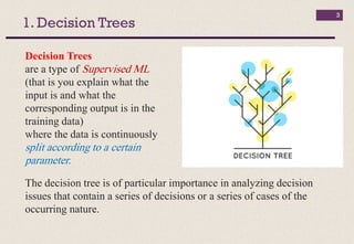
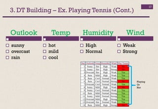
The document outlines the process of building decision trees for machine learning. It discusses key concepts like decision tree structure with root, internal and leaf nodes. It also explains entropy and information gain, which are measures of impurity/purity used to select the best attributes to split nodes on. The example of building a decision tree to predict playing tennis is used throughout to demonstrate these concepts in a step-by-step manner.

1. +

2. Outlines
1. Decision Tree
2. DT-Example
3. DT Building – Ex. Playing Tennis
4. DT Building – Thinking!
5. DT Building – Entropy
6. DT Building – Purity
7. Algorithm for decision tree learning
8. Choose an attribute to partition data
9. Information theory
10. Information Gain
11. Differences between ID3 and C4.5
2

3. 3
1. Decision Trees
Decision Trees
are a type of Supervised ML
(that is you explain what the
input is and what the
corresponding output is in the
training data)
where the data is continuously
split according to a certain
parameter.
The decision tree is of particular importance in analyzing decision
issues that contain a series of decisions or a series of cases of the
occurring nature.

4. 4
2. Decision Tree Example
Body
Temperature
Give Birth
Non-mammals
Non-mammalsMammals
warm
no
cold
yes

5. 5
2. DT-Example (Cont.)
Types of Nodes
Root Node Internal
Node
Leaf Node
that has no incoming
edges and zero or
more outgoing
edges.
each of which has
exactly one incoming
edge and two or more
outgoing edges (circle
symbol).
each of which has
exactly one
incoming edge and
no outgoing edges
(rectangle symbol).
Body
Temperature
Give Birth
Mammals
Non-mammals
Non-mammals

6. 6
• Each leaf node is assigned a class
label.
• The non-terminal nodes (root and
other internal nodes) contain
attribute test conditions to
separate records that have
different characteristics.
• For example, the root node
shown in fig. uses the attribute
Body Temp to separate warm-
blooded from cold-blooded
vertebrates.
Class Label
Test Condition
2. DT-Example (Cont.)

7. 7
3. DT Building – Ex. Playing Tennis
Playing
Or
Not

8. 8
Playing
Or
Not
3. DT Building – Ex. Playing Tennis

9. 9
Playing
Or
Not
Outlook
sunny
overcast
rain
Temp
hot
mild
cool
Humidity
High
Normal
Wind
Weak
Strong
3. DT Building – Ex. Playing Tennis

10. 10
How we can get
DT for this example?
outlook
Humidity
YesNo
sunny
normal
rain
high
Wind
Yes
weak
Yes
No
strong
overcast
3. DT Building – Ex. Playing Tennis

11. 11
4. DT Building – Thinking!
Question 1
Yes No
%50 - %50
Question 2
Yes No
%50 - %50
Temp:
Hot?
Outlook:
sunny?

12. 12
4. DT Building – Thinking! (Cont.)
Question 3
Yes No
Question 4
Yes No
%50 - %50 %50 - %50
%100%100 %50 - %50 %50 - %50

13. 13
5. DT Building – Entropy
Entropy: 𝐸 𝑆 = −𝑃(+) 𝑙𝑜𝑔2 𝑃(+) −𝑃(−) 𝑙𝑜𝑔2 𝑃(−) bits
Or Entropy: 𝐸 𝑆 = − σ𝑖=1
𝑘
𝑝𝑖 𝑙𝑜𝑔2 (𝑝𝑖)
- 𝑆 : subset of training examples
- 𝑃(+) 𝑎𝑛𝑑 𝑃(−): # of positive and # of negative examples in 𝑆
• Interpretation : assume item 𝑋 belongs to 𝑆
- How many bits need to tell if 𝑋 positive or negative
Entropy:
• it relates to machine learning,
• is a measure of the randomness in the information
being processed.

14. 14
0 ≤ 𝐸𝑛𝑡𝑟𝑜𝑝𝑦 ≤ 1
5. DT Building – Entropy (Cont.)
1 2 3
4 5 6
• Impure (4 yes / 4 no)
• E 𝑆 = −
4
8
𝑙𝑜𝑔2
4
8
−
4
8
𝑙𝑜𝑔2
4
8
= 1
• Pure (8 yes / 0 no)
• E 𝑆 = −
8
8
𝑙𝑜𝑔2
8
8
−
0
8
𝑙𝑜𝑔2
0
8
= 0

15. 15
5. DT Building – Entropy (Cont.)
1 4
• Impure (4 yes / 4 no)
• E 𝑆 = −
4
8
𝑙𝑜𝑔2
4
8
−
4
8
𝑙𝑜𝑔2
4
8
= 1
• Pure (8 yes / 0 no)
• E 𝑆 = −
8
8
𝑙𝑜𝑔2
8
8
−
0
8
𝑙𝑜𝑔2
0
8
= 0

16. 16
6. DT Building – Purity
The decision to split at each node is made according to the
metric called purity.
• A node is 100% impure when a node is split evenly 50/50 and
• A node is 100% pure when all of its data belongs to a single class.
• Impure (4 yes / 4 no)
• E 𝑆 = −
4
8
𝑙𝑜𝑔2
4
8
−
4
8
𝑙𝑜𝑔2
4
8
= 1
• Pure (8 yes / 0 no)
• E 𝑆 = −
8
8
𝑙𝑜𝑔2
8
8
−
0
8
𝑙𝑜𝑔2
0
8
= 0

17. 17
Playing
Or
Not
Outlook
sunny
overcast
rain
Temp
hot
mild
cool
Humidity
High
Normal
Wind
Weak
Strong
3. DT Building – Ex. Playing Tennis (Cont.)

18. 18
𝐸 𝑃𝑙𝑎𝑦𝑖𝑛𝑔 = −
9
14
𝑙𝑜𝑔2
9
14
−
5
14
𝑙𝑜𝑔2
5
14
= 0.40978 + 0.53051
= 0.94029
No
Play Play
Playing
Or
Not
3. DT Building – Ex. Playing Tennis (Cont.)

19. 19
Wind
weak strong
𝐸 𝑃𝑙𝑎𝑦𝑖𝑛𝑔 = −
9
14
𝑙𝑜𝑔2
9
14
−
5
14
𝑙𝑜𝑔2
5
14
= 0.40978 + 0.53051
= 0.94029
𝐸 𝑤𝑒𝑎𝑘 = −
6
8
𝑙𝑜𝑔2
6
8
−
2
8
𝑙𝑜𝑔2
2
8
= 0.811
𝐸 𝑠𝑡𝑟𝑜𝑛𝑔 = −
3
6
𝑙𝑜𝑔2
3
6
−
3
6
𝑙𝑜𝑔2
3
6
= 1
No
Play Play
3. DT Building – Ex. Playing Tennis (Cont.)

20. 20
Humidity
high normal
𝐸 𝑃𝑙𝑎𝑦𝑖𝑛𝑔 = −
9
14
𝑙𝑜𝑔2
9
14
−
5
14
𝑙𝑜𝑔2
5
14
= 0.40978 + 0.53051
= 0.94029
𝐸 ℎ𝑖𝑔ℎ = −
3
7
𝑙𝑜𝑔2
3
7
−
4
7
𝑙𝑜𝑔2
4
7
= 0.9854
𝐸 𝑛𝑜𝑟𝑚𝑎𝑙 = −
6
7
𝑙𝑜𝑔2
6
7
−
1
7
𝑙𝑜𝑔2
1
4
= 0.5921
3. DT Building – Ex. Playing Tennis (Cont.)

21. 21
Temp
hot cool
𝐸 𝑃𝑙𝑎𝑦𝑖𝑛𝑔 = −
9
14
𝑙𝑜𝑔2
9
14
−
5
14
𝑙𝑜𝑔2
5
14
= 0.40978 + 0.53051
= 0.94029
𝐸 ℎ𝑜𝑡 = −
2
4
𝑙𝑜𝑔2
2
4
−
2
4
𝑙𝑜𝑔2
2
4
= 1
𝐸 𝑚𝑖𝑙𝑑 = −
4
6
𝑙𝑜𝑔2
4
6
−
2
6
𝑙𝑜𝑔2
2
6
= 0.9185
mild
𝐸 𝑐𝑜𝑜𝑙 = −
3
4
𝑙𝑜𝑔2
3
4
−
1
4
𝑙𝑜𝑔2
1
4
= 0.8114
3. DT Building – Ex. Playing Tennis (Cont.)

22. 22
Outlook
sunny rain
𝐸 𝑃𝑙𝑎𝑦𝑖𝑛𝑔 = −
9
14
𝑙𝑜𝑔2
9
14
−
5
14
𝑙𝑜𝑔2
5
14
= 0.40978 + 0.53051
= 0.94029
𝐸 𝑠𝑢𝑛𝑛𝑦 = −
2
5
𝑙𝑜𝑔2
2
5
−
3
5
𝑙𝑜𝑔2
3
5
= 0.97115
𝐸 𝑜𝑣𝑒𝑟𝑐𝑎𝑠𝑡 = 0
overcast
𝐸 𝑟𝑎𝑖𝑛 = −
3
5
𝑙𝑜𝑔2
3
5
−
2
5
𝑙𝑜𝑔2
2
5
= 0.97115
3. DT Building – Ex. Playing Tennis (Cont.)

23. 23
7. Algorithm for decision tree learning
 Basic algorithm (a greedy divide-and-conquer algorithm)
 Assume attributes are categorical now (continuous attributes
can be handled too)
 Tree is constructed in a top-down recursive manner
 At start, all the training examples are at the root
 Examples are partitioned recursively based on selected
attributes
 Attributes are selected on the basis of an impurity function
(e.g., information gain)
 Conditions for stopping partitioning
 All examples for a given node belong to the same class
 There are no remaining attributes for further partitioning –
majority class is the leaf
 There are no examples left

24. 24
8. Choose an attribute to partition data
 The key to building a decision tree - which attribute to
choose in order to branch.
 The objective is to reduce impurity or uncertainty in
data as much as possible.
 A subset of data is pure if all instances belong to the
same class.
 The heuristic in C4.5 is to choose the attribute with the
maximum Information Gain or Gain Ratio based on
information theory.

25. 25
9. Information theory
 Information theory provides a mathematical basis for measuring the
information content.
 To understand the notion of information, think about it as providing
the answer to a question, for example, whether a coin will come up
heads.
 If one already has a good guess about the answer, then the actual
answer is less informative.
 If one already knows that the coin is rigged so that it will come
with heads with probability 0.99, then a message (advanced
information) about the actual outcome of a flip is worth less than
it would be for a honest coin (50-50).

26. 26
10. Information Gain
 Given a set of examples 𝐷, we first compute its entropy:
 If we make attribute 𝐴𝑖 with 𝑣 values, the root of the
current tree, this will partition 𝐷 into 𝑣 subsets
𝐷1, 𝐷2 … , 𝐷𝑣 . The expected entropy if 𝐴𝑖 is used as the
current root:
𝑒𝑛𝑡𝑟𝑜𝑝𝑦 𝐷 = − σ 𝑗=1
𝑐
P 𝑐𝑗 𝑙𝑜𝑔2 P(𝑐𝑗)
𝑒𝑛𝑡𝑟𝑜𝑝𝑦 𝐴 𝑖
𝐷 = ෍
𝑗=1
𝑣
𝐷𝑗
𝐷
× 𝑒𝑛𝑡𝑟𝑜𝑝𝑦 (𝐷𝑗)

27. 27
10. Information Gain (Cont.)
𝑔𝑎𝑖𝑛 𝐷, 𝐴𝑖 = 𝑒𝑛𝑡𝑟𝑜𝑝𝑦 𝐷 − 𝑒𝑛𝑡𝑟𝑜𝑝𝑦 𝐴 𝑖
(𝐷)
 Information gained by selecting attribute 𝐴𝑖 to
branch or to partition the data is
 We choose the attribute with the highest gain
to branch/split the current tree.
𝑤ℎ𝑒𝑟𝑒;
𝑒𝑛𝑡𝑟𝑜𝑝𝑦 𝐴 𝑖
𝐷 = ෍
𝑗=1
𝑣
𝐷𝑗
𝐷
× 𝑒𝑛𝑡𝑟𝑜𝑝𝑦 (𝐷𝑗)

28. 28
Wind
weak strong
𝐸 𝑃𝑙𝑎𝑦𝑖𝑛𝑔 = 0.94029
𝐸 𝑤𝑒𝑎𝑘 = 0.811 𝐸 𝑠𝑡𝑟𝑜𝑛𝑔 = 1
G 𝑆 , 𝑄 = 𝐸 𝑆 − ෍
𝑖=1
𝑘
𝑝𝑖 × 𝐸(𝑆, 𝑄𝑖)
G 𝑝𝑙𝑎𝑦 , 𝑤𝑖𝑛𝑑 = 0.94029 −
8
14
× 0.811 −
6
14
× 1 = 0.04829
3. DT Building – Ex. Playing Tennis (Cont.)

29. 29
Humidity
high normal
𝐸 𝑃𝑙𝑎𝑦𝑖𝑛𝑔 = 0.94029
𝐸 ℎ𝑖𝑔ℎ = 0.9854 𝐸 𝑛𝑜𝑟𝑚𝑎𝑙 = 0.5921
G 𝑆 , 𝑄 = 𝐸 𝑆 − ෍
𝑖=1
𝑘
𝑝𝑖 × 𝐸(𝑆, 𝑄𝑖)
G 𝑝𝑙𝑎𝑦 , 𝐻𝑢𝑚𝑖𝑑𝑖𝑡𝑦 = 0.94029 −
7
14
× 0.9854 −
7
14
× 0.5921 = 0.15415
3. DT Building – Ex. Playing Tennis (Cont.)

30. 30
Temp
hot cool
𝐸 𝑃𝑙𝑎𝑦𝑖𝑛𝑔 = 0.94029
𝐸 ℎ𝑜𝑡 = 1
𝐸 𝑚𝑖𝑙𝑑 = 0.9185
mild
𝐸 𝑐𝑜𝑜𝑙 = 0.8114
G 𝑆 , 𝑄 = 𝐸 𝑆 − ෍
𝑖=1
𝑘
𝑝𝑖 × 𝐸(𝑆, 𝑄𝑖)
G 𝑝𝑙𝑎𝑦 , 𝑡𝑒𝑚𝑝 = 0.94029 −
4
14
× 1 −
6
14
× 0.9185 −
4
14
× 0.8114 = 0.02919
3. DT Building – Ex. Playing Tennis (Cont.)

31. 31
Outlook
sunny rain
𝐸 𝑃𝑙𝑎𝑦𝑖𝑛𝑔 = 0.94029
𝐸 𝑠𝑢𝑛𝑛𝑦 = 0.97115
𝐸 𝑜𝑣𝑒𝑟𝑐𝑎𝑠𝑡 = 0
overcast
𝐸 𝑟𝑎𝑖𝑛 = 0.97115
G 𝑆 , 𝑄 = 𝐸 𝑆 − ෍
𝑖=1
𝑘
𝑝𝑖 × 𝐸(𝑆, 𝑄𝑖)
G 𝑝𝑙𝑎𝑦 , 𝑜𝑢𝑡𝑙𝑜𝑜𝑘 = 0.94029 −
5
14
× 0.97115 −
4
14
× 0 −
5
14
× 0.97115 = 0.24669
3. DT Building – Ex. Playing Tennis (Cont.)

32. 32
G 𝑝𝑙𝑎𝑦 , 𝑜𝑢𝑡𝑙𝑜𝑜𝑘 = 0.24669
G 𝑝𝑙𝑎𝑦 , 𝑡𝑒𝑚𝑝 = 0.02919
G 𝑝𝑙𝑎𝑦 , 𝐻𝑢𝑚𝑖𝑑𝑖𝑡𝑦 = 0.15415
G 𝑝𝑙𝑎𝑦 , 𝑤𝑖𝑛𝑑 = 0.04829
Playing
Or
Not
3. DT Building – Ex. Playing Tennis (Cont.)

33. 33
G 𝑝𝑙𝑎𝑦 , 𝑜𝑢𝑡𝑙𝑜𝑜𝑘 = 0.24669
Playing
Or
Not
outlook
sunny rain
Yes
overcast
3. DT Building – Ex. Playing Tennis (Cont.)

34. 34
Playing
Or
Not
3. DT Building – Ex. Playing Tennis (Cont.)

35. 35
𝐸 𝑠𝑢𝑛𝑛𝑦 = −
3
5
𝑙𝑜𝑔2
3
5
−
2
5
𝑙𝑜𝑔2
2
5
= 0.444 + 0.532
= 0.976
No
Play Play
Playing
Or
Not
Sunny Set
3. DT Building – Ex. Playing Tennis (Cont.)

36. 36
Wind
weak strong
𝐸 𝑤𝑒𝑎𝑘 = −
1
3
𝑙𝑜𝑔2
1
3
−
2
3
𝑙𝑜𝑔2
2
3
= 0.92
𝐸 𝑠𝑡𝑟𝑜𝑛𝑔 = 1 (𝑖𝑚𝑝𝑢𝑟𝑒 𝑛𝑜𝑑𝑒)
No
Play Play
𝐸 𝑠𝑢𝑛𝑛𝑦 = −
3
5
𝑙𝑜𝑔2
3
5
−
2
5
𝑙𝑜𝑔2
2
5
= 0.444 + 0.532
= 0.976
G 𝑠𝑢𝑛𝑛𝑦 , 𝑤𝑖𝑛𝑑 = 0.976 −
3
5
× 0.92 −
2
5
× 1 = 0.024
3. DT Building – Ex. Playing Tennis (Cont.)

37. 37
𝐸 ℎ𝑖𝑔ℎ = 0 (𝑝𝑢𝑟𝑒 𝑛𝑜𝑑𝑒)
𝐸 𝑛𝑜𝑟𝑚𝑎𝑙 = 0 (pure node)
𝐸 𝑠𝑢𝑛𝑛𝑦 = −
3
5
𝑙𝑜𝑔2
3
5
−
2
5
𝑙𝑜𝑔2
2
5
= 0.444 + 0.532
= 0.976
Humidity
high normal
G 𝑠𝑢𝑛𝑛𝑦 , ℎ𝑢𝑚𝑖𝑑𝑖𝑡𝑦 = 0.976 −
3
5
× 0 −
2
5
× 0 = 0.976
3. DT Building – Ex. Playing Tennis (Cont.)

38. 38
Temp
hot cool
𝐸 ℎ𝑜𝑡 = 0 (pure node)
𝐸 𝑚𝑖𝑙𝑑 = 1 (impure node
mild
𝐸 𝑐𝑜𝑜𝑙 = 0 (pure mode)
G 𝑠𝑢𝑛𝑛𝑦 , 𝑡𝑒𝑚𝑝 = 0.976 −
2
5
× 0 −
2
5
× 1 −
1
5
× 0 = 0.576
𝐸 𝑠𝑢𝑛𝑛𝑦 = −
3
5
𝑙𝑜𝑔2
3
5
−
2
5
𝑙𝑜𝑔2
2
5
= 0.444 + 0.532
= 0.976
3. DT Building – Ex. Playing Tennis (Cont.)

39. 39
Playing
Or
Not
3. DT Building – Ex. Playing Tennis (Cont.)

40. 40
𝐸 𝑟𝑎𝑖𝑛 = −
3
5
𝑙𝑜𝑔2
3
5
−
2
5
𝑙𝑜𝑔2
2
5
= 0.444 + 0.532
= 0.976
No
Play Play
Rain Set
Playing
Or
Not
3. DT Building – Ex. Playing Tennis (Cont.)

41. 41
Wind
weak strong
𝐸 𝑤𝑒𝑎𝑘 = 0 (pure node)
No
Play Play
𝐸 𝑟𝑎𝑖𝑛 = −
3
5
𝑙𝑜𝑔2
3
5
−
2
5
𝑙𝑜𝑔2
2
5
= 0.444 + 0.532
= 0.976
G 𝑟𝑎𝑖𝑛 , 𝑤𝑖𝑛𝑑 = 0.976 −
3
5
× 0.92 −
2
5
× 0 = 0.424
𝐸 𝑠𝑡𝑟𝑜𝑛𝑔 = −
1
3
𝑙𝑜𝑔2
1
3
−
2
3
𝑙𝑜𝑔2
2
3
= 0.92
3. DT Building – Ex. Playing Tennis (Cont.)

42. 42
𝐸 ℎ𝑖𝑔ℎ = 1 (𝑖𝑚𝑝𝑢𝑟𝑒 𝑛𝑜𝑑𝑒)
𝐸 𝑟𝑎𝑖𝑛 = −
3
5
𝑙𝑜𝑔2
3
5
−
2
5
𝑙𝑜𝑔2
2
5
= 0.444 + 0.532
= 0.976
Humidity
high normal
G 𝑟𝑎𝑖𝑛 , ℎ𝑢𝑚𝑖𝑑𝑖𝑡𝑦 = 0.976 −
3
5
× 0.92 −
2
5
× 1 = 0.024
𝐸 𝑛𝑜𝑟𝑚𝑎𝑙 = −
1
3
𝑙𝑜𝑔2
1
3
−
2
3
𝑙𝑜𝑔2
2
3
= 0.92
3. DT Building – Ex. Playing Tennis (Cont.)

43. 43
Temp
No data
hot cool
𝐸 ℎ𝑜𝑡 = no data
mild
𝐸 𝑐𝑜𝑜𝑙 = 1 (impure node)
G 𝑟𝑎𝑖𝑛 , 𝑡𝑒𝑚𝑝 = 0.976 −
3
5
× 0.92 −
2
5
× 1 − 𝑛𝑜 𝑑𝑎𝑡𝑎 = 0.024
𝐸 𝑚𝑖𝑙𝑑 = −
1
3
𝑙𝑜𝑔2
1
3
−
2
3
𝑙𝑜𝑔2
2
3
= 0.92
𝐸 𝑟𝑎𝑖𝑛 = −
3
5
𝑙𝑜𝑔2
3
5
−
2
5
𝑙𝑜𝑔2
2
5
= 0.444 + 0.532
= 0.976
3. DT Building – Ex. Playing Tennis (Cont.)

44. 44
G 𝑠𝑢𝑛𝑛𝑦 , 𝑤𝑖𝑛𝑑 =0.024
outlook
sunny rain
Yes
overcast
G 𝑠𝑢𝑛𝑛𝑦 , ℎ𝑢𝑚𝑖𝑑𝑖𝑡𝑦 = 0.976
G 𝑠𝑢𝑛𝑛𝑦 , 𝑡𝑒𝑚𝑝 =0.576
G 𝑟𝑎𝑖𝑛 , 𝑤𝑖𝑛𝑑 =0.424
G 𝑟𝑎𝑖𝑛 , ℎ𝑢𝑚𝑖𝑑𝑖𝑡𝑦 = 0.024
G 𝑟𝑎𝑖𝑛 , 𝑡𝑒𝑚𝑝 =0.024
3. DT Building – Ex. Playing Tennis (Cont.)

45. 45
outlook
Humidity
YesNo
sunny
normal
rain
high
Yes
overcast
G 𝑟𝑎𝑖𝑛 , 𝑤𝑖𝑛𝑑 =0.424
G 𝑟𝑎𝑖𝑛 , 𝑡𝑒𝑚𝑝 =0.024
3. DT Building – Ex. Playing Tennis (Cont.)

46. 46
outlook
Humidity
YesNo
sunny
normal
rain
high
Wind
Yes
weak
Yes
No
strong
overcast
3. DT Building – Ex. Playing Tennis (Cont.)

47. 47
11. Differences between ID3 and C4.5
ID3 C4.5
Splitting
Criteria
Information
Gain
Ratio Gain
Attribute Type Handles only
categorical
value
Handles both
categorical &
numerical value
Missing Values Do not handle Handle