Download as PDF, PPTX
![Introduction
Concatenation Modeling?
Answer from a logical point of view:
Conc([X|L], L1, [X|L2]) :− Conc(L, L1, L2).
Conc([], L, L).
Conc([a,b], [c,d], L)?
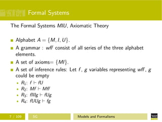
3 / 109 SG Models and Formalisms](https://image.slidesharecdn.com/predicatecalculusv6-151117144424-lva1-app6891/85/Predicate-Calculus-3-320.jpg)
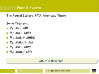


![Prolog Modeling
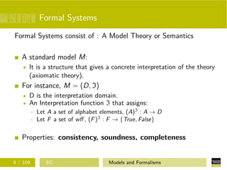
Concatenation Program
Conc([X|L], L1, [X|L2]) :− Conc(L, L1, L2).
Conc([], L, L).
Conc([a,b], [c,d], L)?
85 / 109 SG Models and Formalisms](https://image.slidesharecdn.com/predicatecalculusv6-151117144424-lva1-app6891/85/Predicate-Calculus-93-320.jpg)
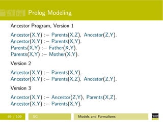
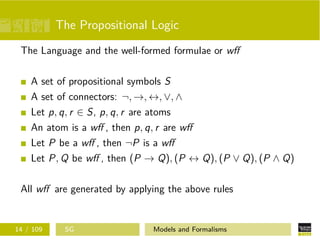
![Prolog Modeling
Eight Queens’ Program
Put(Listdd, Listdg ,Col,8, Result ).
Put(Listdd, Listdg ,Col,Row,Result) :−
Row_1 is Row + 1,
column(I), not(member(I,Col)),
Dd is Row_1 + I, Dg is I − Row_1,
not(member(Dd,Listdd)),
not(member(Dg,Listdg)),
Put([Dd|Listdd ],[ Dg|Listdg ],[ I |Col ], Row_1,[[Row_1,I]|Result]).
Column(1). Column(2). Column(3). Column(4).
Column(5). Column(6). Column(7). Column(8).
88 / 109 SG Models and Formalisms](https://image.slidesharecdn.com/predicatecalculusv6-151117144424-lva1-app6891/85/Predicate-Calculus-96-320.jpg)
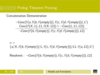
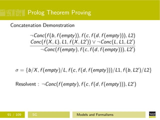
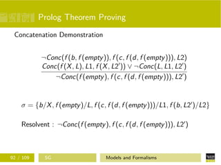
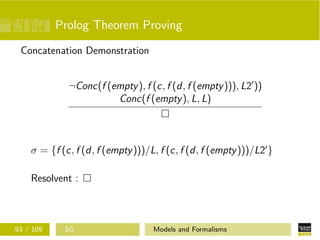
![Prolog Theorem Proving
Concatenation Program
Conc([X|L], L1, [X|L2]) :− Conc(L, L1, L2).
Conc([], L, L).
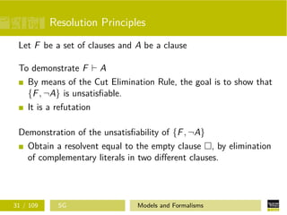
Conc([a,b], [c,d], L)?
∀X, L, L1, L2 (Conc(f (X, L), L1, f (X, L2)) ∨ ¬Conc(L, L1, L2))∧
∀L (Conc(f (empty), L, L)∧
∀L ¬Conc(f (a, f (b, f (empty))), f (c, f (d, f (empty))), L)
89 / 109 SG Models and Formalisms](https://image.slidesharecdn.com/predicatecalculusv6-151117144424-lva1-app6891/85/Predicate-Calculus-97-320.jpg)


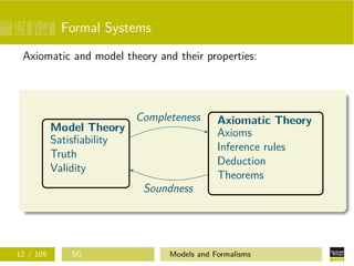
The document discusses models and formalisms in logic. It introduces formal systems as consisting of an axiomatic theory, symbols for constructing formulas, grammar rules, axioms, inference rules, and properties like consistency. Propositional and predicate logic are examined, including their model theories, axiomatic theories, properties like completeness and soundness, and resolution principles. Normal forms and the resolution rule are defined as ways to deduce theorems in a formal system.