Download as PDF, PPTX


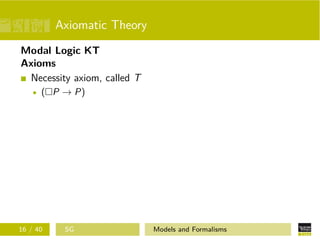


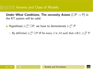
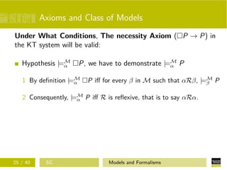
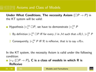

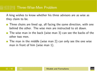


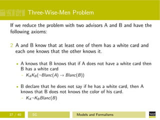

![Three-Wise-Men Problem
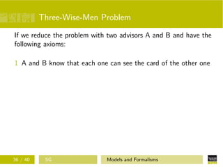
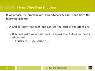
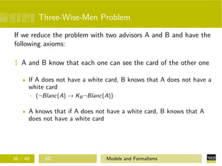
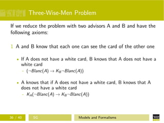
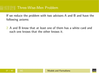
If we can reduce the problem with two advisors and have the
following axioms:
KA(¬Blanc(A) → KB¬Blanc(A)) [1]
38 / 40 SG Models and Formalisms](https://image.slidesharecdn.com/modallogic-151007162913-lva1-app6892/85/Modal-Logic-88-320.jpg)
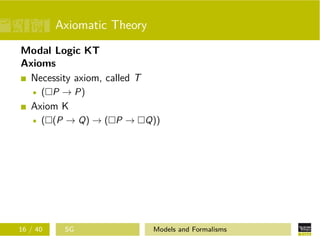
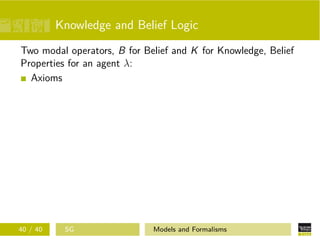
![Three-Wise-Men Problem
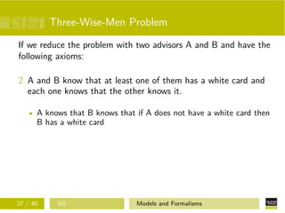
If we can reduce the problem with two advisors and have the
following axioms:
KA(¬Blanc(A) → KB¬Blanc(A)) [1]
KAKB(¬Blanc(A) → Blanc(B)) [2]
KA¬KBBlanc(B) [3]
38 / 40 SG Models and Formalisms](https://image.slidesharecdn.com/modallogic-151007162913-lva1-app6892/85/Modal-Logic-89-320.jpg)
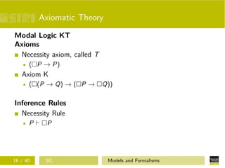
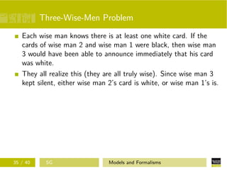
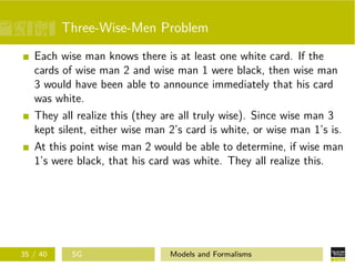
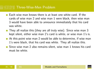
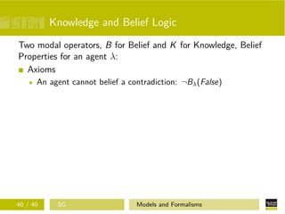
![Three-Wise-Men Problem
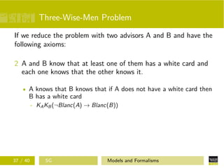
If we can reduce the problem with two advisors and have the
following axioms:
KA(¬Blanc(A) → KB¬Blanc(A)) [1]
KAKB(¬Blanc(A) → Blanc(B)) [2]
KA¬KBBlanc(B) [3]
38 / 40 SG Models and Formalisms](https://image.slidesharecdn.com/modallogic-151007162913-lva1-app6892/85/Modal-Logic-90-320.jpg)
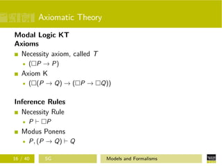
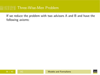
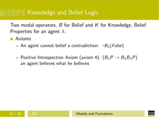
![Three-Wise-Men Problem
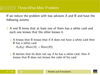
If we can reduce the problem with two advisors and have the
following axioms:
KA(¬Blanc(A) → KB¬Blanc(A)) [1]
KAKB(¬Blanc(A) → Blanc(B)) [2]
KA¬KBBlanc(B) [3]
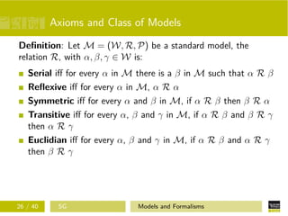
[1] (KA(¬Blanc(A) → KB¬Blanc(A)) (KλP → P) [Axiom2]
[4] (¬Blanc(A) → KB¬Blanc(A))
38 / 40 SG Models and Formalisms](https://image.slidesharecdn.com/modallogic-151007162913-lva1-app6892/85/Modal-Logic-91-320.jpg)
![Three-Wise-Men Problem
If we can reduce the problem with two advisors and have the
following axioms:
KA(¬Blanc(A) → KB¬Blanc(A)) [1]
KAKB(¬Blanc(A) → Blanc(B)) [2]
KA¬KBBlanc(B) [3]
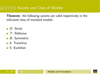
[1] (KA(¬Blanc(A) → KB¬Blanc(A)) (KλP → P) [Axiom2]
[4] (¬Blanc(A) → KB¬Blanc(A))
[2] KAKB(¬Blanc(A) → Blanc(B)) (KλP → P) [Axiom2]
[5] (KB(¬Blanc(A) → Blanc(B))
(Kλ(P → Q) → (KλP → KλQ)) [Axiom1]
[6] (KB¬Blanc(A) → KBBlanc(B))
38 / 40 SG Models and Formalisms](https://image.slidesharecdn.com/modallogic-151007162913-lva1-app6892/85/Modal-Logic-92-320.jpg)
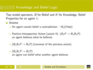
![Three-Wise-Men Problem
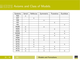
Omniscience
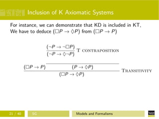
Contraposition
Transitivity
[4] (¬Blanc(A) → KB¬Blanc(A))
(KB¬Blanc(A) → KBBlanc(B)) [6]
[7] (¬Blanc(A) → KBBlanc(B))
[8] (¬KBBlanc(B) → Blanc(A))
[1] [2] [4] [5]
[9] (KA(¬KBBlanc(B) → Blanc(A)))
(Kλ(P → Q) → (KλP → KλQ)) [Axiom1]
(KA¬KBBlanc(A) → KABlanc(A))
KA¬KBBlanc(B) [3]
[11] KABlanc(A)
39 / 40 SG Models and Formalisms](https://image.slidesharecdn.com/modallogic-151007162913-lva1-app6892/85/Modal-Logic-93-320.jpg)

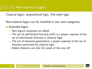
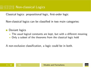
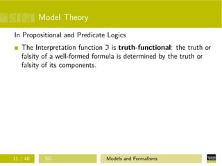
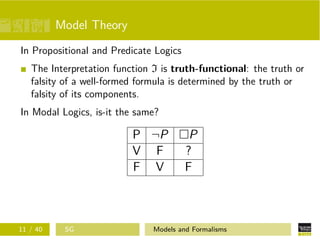
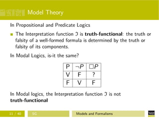
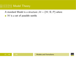
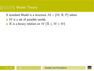
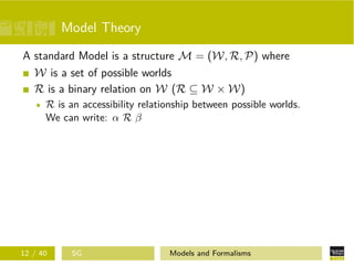
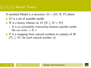
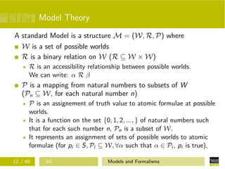
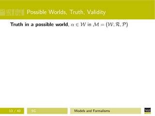
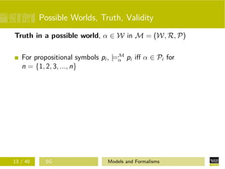
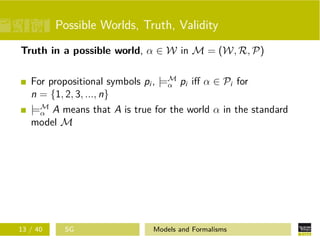
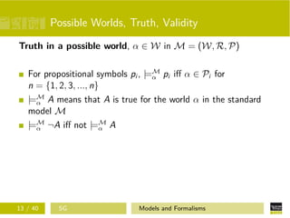
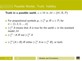
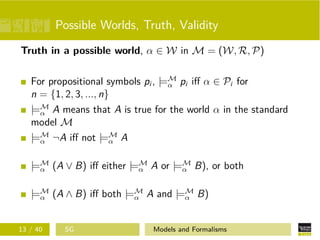
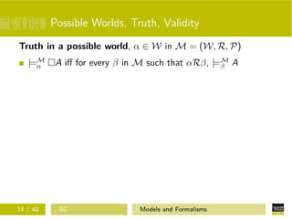
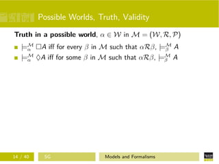
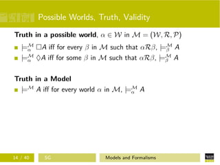
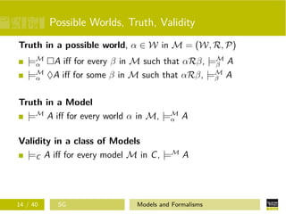
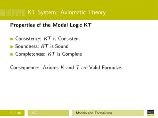
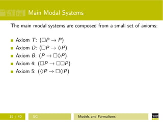
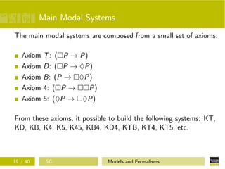
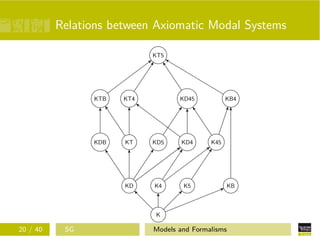
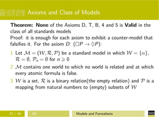
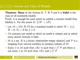
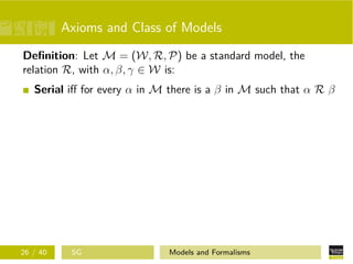
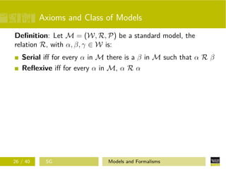
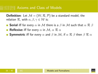
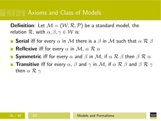
This document discusses modal logics and formalisms. It defines modal logics as logics that add new logical constants like necessity (□) and possibility (◇) to classical logic. It describes how modal logics can be classified based on whether they are extended logics that add new well-formed formulas or deviant logics that interpret the usual logical constants differently. The document then focuses on modal logics, defining their language and providing details on their model theory using possible world semantics. It discusses truth in possible worlds and models. It also describes several axiomatic modal systems and the relationships between them, and examines the classes of models validated by different axioms.