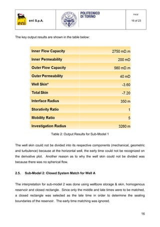
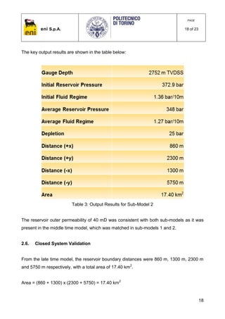
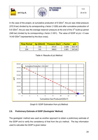
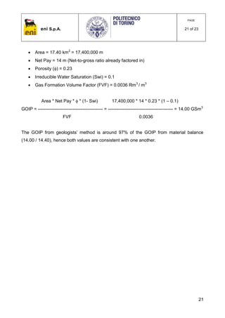
The document discusses well testing interpretation for a gas reservoir case study. Bottom-hole pressure and rate data from April 2012 to December 2013 for Well A was input into interpretation software. A build-up period was interpreted to estimate reservoir properties. The average reservoir pressure was found to be 348 bar, with an average permeability of 40 mD for Well A. Interference from nearby wells prevented using data after December 2013. A preliminary estimate of original gas in place was 14.40 GSm3 using material balance methods.

1. eni S.p.A.
PAGE
1 of 23
1
Well Testing for Reservoir Management: A Case Study
2014-2015 Master in Petroleum Engineering and Operations
eni Stage Thesis
AUTHOR
Pratik Nityanand Rao RESM / IPET
Date: 15/10/2015
eni Stage Department eni Supervisors University Tutor
RESM / IPET Mr. E. Beretta
RESM / IPET Mr. G. Tripaldi
Prof. F. Verga

2. eni S.p.A.
PAGE
2 of 23
2
Management Summary
The scope of this project was to verify when well testing interpretation of permanent
gauges was feasible and helpful for reservoir monitoring and to provide a preliminary
reservoir characterization for the case study.
For the project, bottom-hole pressures from downhole gauges and field rates (April 2012 –
December 2013) were obtained from the well archives and inputted into Interpret in order
to achieve an interpretation of a selected build-up period.
The bottom-hole pressures and field rates were used from the aforementioned time period
because after December 2013, interference from other wells were occurring, therefore the
data post December 2013 could not be interpreted an was rejected.
From the interpretation of a single build-up period, the wellbore & bulk reservoir properties
along with the reservoir boundary distances were identified, which were subsequently
used to calculate a preliminary estimate of the gas originally in place (GOIP) using the
material balance and geologist’ method.

3. eni S.p.A.
PAGE
3 of 23
3
Conclusions
 The standard approach for build-up and drawdown interpretation could not be
applied to this case study due to inadequate build-up and drawdown durations,
hence an alternative workflow was implemented.
 The average reservoir pressure at gauge depth (2752 m TVDss) after 0.6 GSm3
of
cumulative production resulted to be 348 bar, with a corresponding depletion of
about 25 bar (initial reservoir pressure = 372.9 bar from WFT / RFT).
 The average effective gas permeability for Well A was 40 mD.
 The skin was about -4, which indicates that the well is not damaged.
 The skin could not be sub-divided into its components (mechanical, geometric and
turbulence) because at the horizontal well, early time cannot be recognised on the
derivative plot.
 The preliminary estimate of GOIP was 14.40 GSm3
(from material balance) after
cumulative production of 0.6 GSm3
.

4. eni S.p.A.
PAGE
4 of 23
4
List of Contents
1. PROJECT BACKGROUND......................................................................................................6
1.1. PROJECT SCOPE.........................................................................................................................................6
1.2. INTERFERENCE FROM NEARBY WELLS ..............................................................................................6
1.3. STANDARD APPROACH TO WELL TESTING INTERPRETATION......................................................7
1.4. ALTERNATIVE APPROACH TO WELL TESTING INTERPRETATION ...............................................8
2. DISCUSSION OF THE CASE STUDY ..................................................................................10
2.1. GENERAL INFORMATION OF THE FIELD..........................................................................................10
2.2. PRODUCTION HISTORY ..........................................................................................................................12
2.3. COMPARISON OF BUILD-UPS FOR WELL A .......................................................................................13
2.4. SUB-MODEL 1 – RADIAL COMPOSITE MATCH FOR WELL A ..........................................................14
2.5. SUB-MODEL 2 – CLOSED SYSTEM MATCH FOR WELL A .................................................................16
2.6. CLOSED SYSTEM VALIDATION.............................................................................................................18
2.7. PRELIMINARY ESTIMATE OF GOIP (P/Z METHOD)..........................................................................19
2.8. PRELIMINARY ESTIMATE OF GOIP (GEOLOGISTS’ METHOD) .....................................................20
3. CONCLUSIONS........................................................................................................................22
4. BIBLIOGRAPHY .....................................................................................................................23

5. eni S.p.A.
PAGE
5 of 23
5
List of the Figures
FIGURE 1: DRAWDOWN SCENARIO ......................................................................................................................................6
FIGURE 2: BUILD-UP SCENARIO ..........................................................................................................................................7
FIGURE 3: CLOSED RECTANGULAR RESERVOIR...................................................................................................................7
FIGURE 4: ALTERNATIVE APPROACH...................................................................................................................................9
FIGURE 5: DOWN-HOLE CONFIGURATION OF WELL A ......................................................................................................11
FIGURE 6: DOWN-HOLE CONFIGURATION OF WELL B.......................................................................................................12
FIGURE 7: CLOSED RECTANGULAR RESERVOIR VALIDATION............................................................................................19
FIGURE 8: P/Z METHOD......................................................................................................................................................19
List of the Tables
TABLE 1: GENERAL INFORMATION OF THE FIELD (RESERVOIR & FLUID DATA, WELLS A & B DATA) .............................10
TABLE 2: OUTPUT RESULTS FOR SUB-MODEL 1................................................................................................................16
TABLE 3: OUTPUT RESULTS FOR SUB-MODEL 2................................................................................................................18
TABLE 4: RESULTS OF P/Z METHOD...................................................................................................................................20
List of the Graphs
GRAPH 1: PRESSURE AND DERIVATIVE CURVES OF DRAWDOWN & BUILD-UP FOR STANDARD APPROACH .......................8
GRAPH 2: PRESSURE & DERIVATIVE CURVES OF DRAWDOWN & BUILD-UP FOR ALTERNATIVE APPROACH ......................8
GRAPH 3: PRODUCTION HISTORY FOR WELLS A & B........................................................................................................13
GRAPH 4: COMPARISON OF BUILD-UPS FOR WELL A........................................................................................................14
GRAPH 5: LOG-LOG MATCH OF SUB-MODEL 1 .................................................................................................................15
GRAPH 6: PRESSURE HISTORY MATCH OF SUB-MODEL 1 .................................................................................................15
GRAPH 7: LOG-LOG MATCH OF SUB-MODEL 2 .................................................................................................................17
GRAPH 8: PRESSURE HISTORY MATCH OF SUB-MODEL 2 .................................................................................................17
GRAPH 9: GOIP ESTIMATION FROM P/Z METHOD..............................................................................................................20

6. eni S.p.A.
PAGE
6 of 23
6
1. PROJECT BACKGROUND
1.1. Project Scope
The scope of this project was to verify when well testing interpretation of permanent
gauges was feasible and helpful for reservoir monitoring and to provide a preliminary
reservoir characterization for the case study. The following key points were addressed
during the project:
 Interference from nearby wells
 Inadequate build-up and drawdown periods
 Complexity of the interpretation model
1.2. Interference from Nearby Wells
For the drawdown scenario (please see figure below), there are 5 wells that are open and
producing at a constant rate. Each well is only producing within its drainage area and is
able to defend it from being encroached upon by the other 4 wells, hence the interpretation
is usually more reliable.
Figure 1: Drawdown Scenario
For the build-up scenario (please see figure in next page), there are 4 wells that are open
and producing at a constant rate and 1 well which is shut-in and therefore not producing.

7. eni S.p.A.
PAGE
7 of 23
7
In this case, the 4 open wells initially deplete their respective drainage areas and then
invade that of the shut-in well. This phenomenon is known as interference from nearby
wells and the build-up late time models are usually disturbed, hence they cannot be
interpreted.
Figure 2: Build-Up Scenario
1.3. Standard Approach for Well Testing Interpretation
The standard approach for well testing interpretation is performed for long build-up and
drawdown periods. If a closed rectangular reservoir is considered, the reservoir response
shows IARF (Infinite Acting Radial Flow) behaviour before all the barriers are reached.
The duration of the radial flow is a function of the well location inside the rectangular area.
Figure 3: Closed Rectangular Reservoir

8. eni S.p.A.
PAGE
8 of 23
8
In the drawdown derivative, when all sealing boundaries are reached, both the pressure
and deritvative curve follow a slope of 1 (straight line). For the build-up derivative, when
all sealing boundaries are reached, the reservoir pressure tends to stabilise at the average
reservoir pressure and therefore the curve drops.
Graph 1: Pressure and Derivative Curves of Drawdown & Build-Up for Standard Approach
1.4. Alternative Approach for Well Testing Interpretation
The alternative approach for well testing interpretation is performed during short or
inadequate build-up and drawdown durations. The data for this case is very difficult to
interpret and the model is complicated, hence it is divided into 2 sub-models.
Graph 2: Pressure & Derivative Curves of Drawdown & Build-Up for Alternative Approach

9. eni S.p.A.
PAGE
9 of 23
9
Figure 4: Alternative Approach
Prior to commencing on the interpretation of the separate sub-models, it is compulsory to
set the initial reservoir pressure, which can be obtained from the WFT/RFT. Then, using a
build-up derivative, an interpretation is run in order to get a log-log plot which is
subsequently used to match the early and middle times for estimation of wellbore and bulk
reservoir properties. The next step is to match the middle and late times for estimation of
the reservoir boundaries.
If the simulated bottom-hole pressures do not match the actual bottom-hole pressures, the
boundary distances are to be modified and the simulation is restarted. In the event of both
bottom-hole pressures being matched, the variable skin is applied to correct the non-Darcy
skin and therefore improve the drawdown matching.
The 2 sub-models had to be consistent with the reservoir outer permeability because this
value was present in the middle time model, which was used in both sub-models.

10. eni S.p.A.
PAGE
10 of 23
10
2. DISCUSSION OF THE CASE STUDY
2.1. General Information of the Field
Table 1: General Information of the Field (Reservoir & Fluid Data, Wells A and B Data)
Well A is a single producer and has a horizontal gravel pack along with 7” – 5.5”
completion. The gauge depth is 2752 m TVDSS and top and bottom gravel are at 2769 m
TVDSS and 2779 m TVDSS respectively. The angle of well A is 85-89 degrees at the
target, with a horizontal net length (Lw) of 200 m.
The geological data for well A was obtained between the top and bottom gravel, between
3104 m MD and 3320 m MD respectively. The lithology of this region was predominantly
high quality sandstone (Φ > 24%) along with poor quality sandstone (Φ = 9% – 15%) near
the top gravel.

11. eni S.p.A.
PAGE
11 of 23
11
Figure 5: Down-Hole Configuration of Well A
Well B is also a single producer and has a horizontal gravel pack along with 7” – 5.5”
completion. The gauge depth is 2753 m TVDSS and top and bottom gravel are at 2785 m
TVDSS and 2798 m TVDSS respectively. The angle of well B is 85 degrees at the target,
with a horizontal net length (Lw) of 130 m.
The geological data for well B was obtained between the top and bottom gravel, between
3404 m MD and 3557 m MD respectively. The lithology of this region was a mixture of
shale and sandstone that ranged from high to poor quality. Near the bottom gravel, the
lithology was all high quality sandstone with porosity being greater than 24%.

12. eni S.p.A.
PAGE
12 of 23
12
Figure 6: Down-Hole Configuration of Well B
2.2. Production History
The production history for wells A and B was split into two sections: field production for
well A and alternating production for wells A and B. Due to an electrical failure in the
gauges during the first 6 months of production, the bottom-hole pressures of well A could
not be recorded, however the initial reservoir pressure at gauge depth was 372.9 bar.
There were 3 distinct build-up periods when well A was shut-in, where the reservoir
pressure equilibrated to 348 bar (average reservoir pressure) at the end of the 3rd
build-up
period. Well B was shut-in for this entire time period, except being open for around 3-4
days during its clean-up phase.

13. eni S.p.A.
PAGE
13 of 23
13
Graph 3: Production History for Wells A & B
In section 2, there is alternating production for wells A & B, whereby when well A is shut-in
(production = 0), well B is open and producing and vice versa. However, during the build-
up of well A (when well B is production), its bottom-hole pressure initially increases and
then instead of stabilizing, it starts to decrease. The same can be seen when well B is in
build-up and well A in production. This proves that interference from wells is occurring and
therefore, interpretation of data (build-up and drawdown) is not possible for either wells.
Hence, this information was not used for the project and only that in section 1 (field
production for well A) was considered.
2.3. Comparison of Build-Ups for Well A
The bottom-hole pressures and field rates for well A were tabulated on Microsoft Excel and
then inputted into Interpret, where the production and pressure histories were displayed in
a graphical form. Flow periods were defined and each build-up period was selected to be
interpreted on the log-log plot to determine their consistency. All the build-up periods

14. eni S.p.A.
PAGE
14 of 23
14
followed more or less the same trend (horizontal well) hence, they were consistent with
one another.
Graph 4: Comparison of Build-Ups for Well A
2.4. Sub-Model 1: Radial Composite Match for Well A
Since the log-log plot for all 3 build-ups displayed a shape that was pertaining to a
horizontal well, this model was used for matching the real data. The effective horizontal
producing length (Lw), for which the simulated data would match the real data, was a lot
greater than the actual Lw for well A (200 m). This was unrealistic, hence the vertical well
model was used for the matching on the log-log plot.
The interpretation for the first sub-model was done using wellbore storage & skin, radial
composite and infinite lateral extent. Since only the early and middle time models were to
be matched, the late time selected was infinite lateral extent, whereby the boundaries were
not defined. From the log-log match, the early and middle times are well honoured.

15. eni S.p.A.
PAGE
15 of 23
15
Graph 5: Log-Log Match of Sub-Model 1
The first build-up period was analysed for this interpretation, and from the pressure history
match, all 3 build-ups were well honoured.
Graph 6: Pressure History Match of Sub-Model 1

16. eni S.p.A.
PAGE
16 of 23
16
The key output results are shown in the table below:
Table 2: Output Results for Sub-Model 1
The well skin could not be divided into its respective components (mechanical, geometric
and turbulence) because at the horizontal well, the early time could not be recognized on
the derivative plot. Another reason as to why the well skin could not be divided was
because there was no spherical flow.
2.5. Sub-Model 2: Closed System Match for Well A
The interpretation for sub-model 2 was done using wellbore storage & skin, homogenous
reservoir and closed rectangle. Since only the middle and late times were to be matched,
a closed rectangle was selected as the late time in order to determine the sealing
boundaries of the reservoir. The early time matching was ignored.

17. eni S.p.A.
PAGE
17 of 23
17
Graph 7: Log-Log Match of Sub-Model 2
As with the first sub-model, the first build-up period was analysed for this interpretation,
and from the pressure history match, all 3 build-ups were well honoured.
Graph 8: Pressure History Match of Sub-Model 2

18. eni S.p.A.
PAGE
18 of 23
18
The key output results are shown in the table below:
Table 3: Output Results for Sub-Model 2
The reservoir outer permeability of 40 mD was consistent with both sub-models as it was
present in the middle time model, which was matched in sub-models 1 and 2.
2.6. Closed System Validation
From the late time model, the reservoir boundary distances were 860 m, 1300 m, 2300 m
and 5750 m respectively, with a total area of 17.40 km2
.
Area = (860 + 1300) x (2300 + 5750) = 17.40 km2

19. eni S.p.A.
PAGE
19 of 23
19
Figure 7: Closed Rectangular Reservoir Validation
2.7. Preliminary Estimate of GOIP (p/z Method)
A preliminary estimate of the gas originally in place (GOIP) was done using the p/z
method, where the GOIP (G) was obtained by plotting a graph of p/z vs Gp, extrapolating
the line to the point where p/z = 0 and reading the value of G on the x axis.
Figure 8: p/z Method

20. eni S.p.A.
PAGE
20 of 23
20
In the case of the project, at cumulative production of 0 GSm3
, the p/z was initial pressure
(372.9 bar) divided by its corresponding z factor (1.028) and after cumulative production of
0.6 GSm3
, the p/z was the average reservoir pressure at the end of the 3rd
build-up period
(348 bar) divided by its corresponding z factor (1.001). The value of GOIP at p/z = 0 was
14.40 GSm3
(represented by the blue cross).
Flow Period Gp (GSm3) Pressure (bar) z Factor p/z
0 0.0 372.9 1.028 362.74
234 0.6 348.0 1.001 347.64
Table 4: Results of p/z Method
Graph 9: GOIP Estimation from p/z Method
2.8. Preliminary Estimate of GOIP (Geologists’ Method)
The geologists’ method was used as another approach to obtain a preliminary estimate of
the GOIP and to verify the consistency of that from the p/z method. The key information
used to calculate the GOIP is given below:

21. eni S.p.A.
PAGE
21 of 23
21
 Area = 17.40 km2
= 17,400,000 m
 Net Pay = 14 m (Net-to-gross ratio already factored in)
 Porosity () = 0.23
 Irreducible Water Saturation (Swi) = 0.1
 Gas Formation Volume Factor (FVF) = 0.0036 Rm3
/ m3
Area * Net Pay *  * (1- Swi) 17,400,000 * 14 * 0.23 * (1 – 0.1)
GOIP = ------------------------------------------- = ------------------------------------------- = 14.00 GSm3
FVF 0.0036
The GOIP from geologists’ method is around 97% of the GOIP from material balance
(14.00 / 14.40), hence both values are consistent with one another.

22. eni S.p.A.
PAGE
22 of 23
22
3. CONCLUSIONS
Taking into account the 3 key points mentioned earlier in the report, each one had a
solution which was implemented in the case study.
The solution for interference from nearby wells was to obtain a long drawdown acquisition
at constant rate, therefore the well testing interpretation was performed on data that was
unaffected by interference i.e. field production of well A only. This was because the build-
up and drawdown data for alternating production of wells A and B could not be interpreted
on the software.
The solution for inadequate build-up and drawdown durations was to implement an
alternative approach for interpretation, which required a reliable value of initial reservoir
pressure from WFT / RFT and at least one build-up acquisition. The initial reservoir
pressure obtained was 372.9 bar and the 1st
build-up period from field production of well A
was analyzed.
The solution for complexity of the model was to divide it into 2 sub-models and interpret
each separately. The wellbore and bulk reservoir properties were obtained from sub-
model 1, by matching the early and middle times and the boundary distances were
obtained from sub-model 2, by matching the middle and late times. From this information,
a preliminary estimate of the GOIP could be calculated using the material balance and
geologists’ method.
Another solution for the model complexity was to use numerical well testing software,
however this was not possible because the software is used for complex systems,
complex geological features and multiphase flow, therefore this was beyond the scope of
the project.

23. eni S.p.A.
PAGE
23 of 23
23
4. BIBLIOGRAPHY
[1] Gas Well Testing Handbook, Amanat U. Chaudhry
[2] Dynamic Data Analysis, Olivier Houze, Didier Viturat & Ole S. Fjaere
[3] Introductory Well Testing, Tom Aage Jelmert
[4] Politecnico di Torino 2nd
Level Master 2014-15 Notes, Prof. Francesca Verga
[5] Well Testing Analysis in Practice, Prof. Alain C. Gringarten