This document is an introduction to topological vector spaces written by Oliver Taylor for his MA-M00 project at Swansea University. It begins with brief histories of functional analysis and topological vector spaces. Fundamental concepts from vector spaces, convexity, and topology are then introduced. These include definitions of vector spaces, convex sets, open sets, neighborhoods, and topological spaces. The interactions between topology, convexity, and vector space structures are discussed. Finally, topological vector spaces are defined as vector spaces endowed with a topology compatible with the algebraic operations. Examples and applications are discussed in the last section.
![1 Introduction
1.1 A brief history of Functional Analysis and Topo-
logical Vector Spaces
The first study of Topological Vector Spaces started between 1920 and 1930,
which is when the general theory was established. Much of what is stud-
ied has its roots in functional analysis and so it could be said that much of
the groundwork had already been laid in the 20th
Century and perhaps ear-
lier. This dissertation discusses some preliminary notions and first examples
within topological vector spaces. More detailed history, on this and other
topics, can be found using [1] [Bourbaki], from which the above facts were
taken.
1.2 Motivation
In this dissertation we want to get a grounding in some areas of the theory of
topological vector spaces. We begin this by collecting together concepts from
vector spaces in 2.1, and convexity and topology in 2.2 and 2.3 respectively.
From 2.3 comes the notion of neighbourhoods, which we shall see is funda-
mental in understanding topologies. In particular we shall look at some of
the interactions between the topology and convexity and the effects it has on
the set we are working with. Then of crucial importance, which comes in
2.4, is the fact that taking a set with a topology that is compatible with the
continuous algebraic operations of the set yields a topological vector space.
From here we look more deeply at the interaction between neighbourhoods
and the topology before introducing seminorms. We find that seminorms
can be used to create topologies on sets, and then we shall finally look at
2](https://image.slidesharecdn.com/83ed9392-09ad-4275-b5fe-da6bc7d962f4-150716125805-lva1-app6891/75/Topological_Vector_Spaces_FINAL_DRAFT-3-2048.jpg)
![Remark 2.1.2. We note here that K is used to denote either R or C. In
most cases we consider in this dissertation, there is no difference between
the real and complex case. We shall only specify the use of real or complex
numbers when clarity is needed or when the cases differ significantly.
We take the following two definitions from [3] [page 4]. These are helpful
in understanding the structure of vector spaces.
Definition 2.1.3. Let X be a K vector space. We call a subset L ⊂ X
linearly independent if for every finite linear combination
λ1x1 + λ2x2 + ... + λkxk = 0, xj ∈ L, xj = xi for j = i, λj ∈ K,
it follows that
λ1 = λ2 = ... = λk = 0, k ∈ N.
Remark 2.1.4. The above definition is taken for the finite case. It does also
hold in the case of the vector space being infinite dimensional.
Definition 2.1.5. Let X be a K-vector space and W ⊂ X be a subset of X.
We call the set of all finite linear combinations
m
k=1
λkwk, λk ∈ K, wk ∈ W, 1 ≤ k ≤ m, m ∈ N
the span, spanW or linear hull of W, i.e.:
spanW = {x ∈ X x =
m
k=1
λkwk for some λk ∈ K, wk ∈ W, 1 ≤ k ≤ m, m ∈ N}.
Definition 2.1.6. A linearly independent spanning (sub)set of a vector
space is called a basis, or more precisely, an algebraic basis or Hamel basis.
5](https://image.slidesharecdn.com/83ed9392-09ad-4275-b5fe-da6bc7d962f4-150716125805-lva1-app6891/75/Topological_Vector_Spaces_FINAL_DRAFT-6-2048.jpg)
![2.2 Convexity
We now look to understand convexity of a set. This notion will be important
in understanding the structure (and later the topology - which we have yet
to formally define) of a set.
Definition 2.2.1. Let V be a K-vector space, X ⊂ V be a subset, and let
x1 and x2 ∈ X. Then X is said to be convex if
((1 − λ)x1 + λx2) ∈ X, for λ ∈ [0, 1].
For a clearer idea of what is meant by convexity, we have the following.
Figure 1: Convex Set
Figure 1 is a trivial example within the Euclidean 2-dimensional space,
showing that any two points can be “joined” by a straight line contained
entirely within the set. This notion is not limited to the Euclidean space;
it holds for any set satisfying the properties of convexity, but it is easier to
understand in the context of Euclidean spaces, hence the above example.
Figure 1 was obtained from [8].
Definition 2.2.2. A subset X of a vector space V is said to be absolutely convex
or balanced if it is convex and there is a subset W in X such that for
w ∈ W and λ ∈ K, when |λ| ≤ 1, we have that
6](https://image.slidesharecdn.com/83ed9392-09ad-4275-b5fe-da6bc7d962f4-150716125805-lva1-app6891/75/Topological_Vector_Spaces_FINAL_DRAFT-7-2048.jpg)
![λW ⊂ W
where,
λW := λw w ∈ W .
Definition 2.2.3. A convex subset X of a vector space V is said to be
absorbent if for all x ∈ V , there is some λ > 0, λ ∈ K, such that x ∈ µX,
where
µX := µx x ∈ X ,
for λ ≤ |µ|, µ ∈ K.
Remark 2.2.4. The intersection of convex sets is convex.
Remark 2.2.5. Vector spaces are, by definition, convex.
From the fact in Remark 2.2.4 and using [7] [page 1], we have the following
definition.
Definition 2.2.6. The convex hull of a given set B, denoted by Conv(B) is
defined to be the intersection of all convex sets containing B.
7](https://image.slidesharecdn.com/83ed9392-09ad-4275-b5fe-da6bc7d962f4-150716125805-lva1-app6891/75/Topological_Vector_Spaces_FINAL_DRAFT-8-2048.jpg)
![2.3 Topology
We now gather some basic ideas from topology, which essentially is concerned
with continuity of functions on sets and their convergence. To understand
the topology of a given set, we must look at open (sub)sets and neighbour-
hoods.
First we must understand the concept of an open set. We start by con-
sidering the case on the real line R and then generalise the definition after
introducing the key definition in this section, the topology. The following
definition of open sets uses material from [2][page 8].
Definition 2.3.1. Let x ∈ R be a point. Let I be an interval (a, b) where
a < b. Then for x ∈ I we have a < x < b and I is called an open set or an
open interval.
Now we introduce a topology. To make sense of the definition, we need
to slightly generalise the idea of Definition 2.3.1, making it somewhat ab-
stract. Later however, we shall generalise the definition of open sets in a
more concrete way.
Definition 2.3.2. A topology OX on a set X is a collection of open (sub)sets,
where the following properties are satisfied:
X is an open set, (2.3.1)
∅ is an open set, (2.3.2)
The unions of open sets are open, (2.3.3)
The finite intersections of open sets are open. (2.3.4)
A set X satisfying such properties is known as a topological space.
8](https://image.slidesharecdn.com/83ed9392-09ad-4275-b5fe-da6bc7d962f4-150716125805-lva1-app6891/75/Topological_Vector_Spaces_FINAL_DRAFT-9-2048.jpg)
![Remark 2.3.3. A topology on a set is not necessarily unique; there may
exist several topologies on a set. In fact, we can often topologise a set in a
chosen way to yield certain results or to simplify our calculations.
Definition 2.3.4. Let X be a topological space, and let x ∈ X be a point.
The set U is called a neighbourhood of x if there exists an open set Y , with
x ∈ Y ⊂ U.
We denote by Ux the set of all neighbourhoods of the point x ∈ X. Ux
has the following properties:
x ∈ U for all U ∈ Ux. (2.3.5)
If U ∈ Ux and U ∈ Ux, then U ∩ U ∈ Ux. (2.3.6)
If U ∈ Ux and U ⊂ U , then U ∈ Ux. (2.3.7)
If U ∈ Ux, there exists U ∈ Ux with U ∈ Ux for all x ∈ U .
(2.3.8)
We now generalise the idea of open sets into something less abstract using
neighbourhoods.
The following definition of open sets can be found in [6][page 4].
Definition 2.3.5. If E is a topological space and U a subset, then U is
called open (in E) if, for each p ∈ U, U is a neighbourhood of p.
Definition 2.3.6. A topological space X is called Hausdorff or separated if
any two distinct points have disjoint neighbourhoods.
Definition 2.3.7. Let X be a topological space with a topology OX. A
collection of open sets O X ⊂ OX is called a base for OX if every open set is
a union of elements of O X.
9](https://image.slidesharecdn.com/83ed9392-09ad-4275-b5fe-da6bc7d962f4-150716125805-lva1-app6891/75/Topological_Vector_Spaces_FINAL_DRAFT-10-2048.jpg)
![Remark 2.3.8. We must note here that bases in this sense are not the same
as bases of vector spaces (i.e.: a linearly independent spanning (sub)set of
vectors).
Definition 2.3.9. Let X be a topological space, where we have two topolo-
gies defined on it, OX and O X. We say that OX is finer than O X (or O X
is coarser than OX) if every set that is open in O X is also open in OX, i.e.:
O X ⊂ OX.
Definition 2.3.10. Let f : A → B be a function, and let S be a subset of
B. Then the pre-image of S under f is the subset of A defined by
f−1
(S) = {x ∈ A f(x) ∈ S},
which consists of all points which are mapped to S by f.
Remark 2.3.11. So that no confusion may arise, we will specify when talk-
ing about inverses of functions explicitly. Otherwise, when not specified,
we shall assume that f−1
denotes the pre-image of f.
We now need to define an open mapping, as what follows is a power-
ful theorem that is helpful in understanding continuity of mappings when
working with open sets and topological spaces. This definition expands on
material found at [9] the Wolfram MathWorld website.
Definition 2.3.12. Let X and Y be topological spaces. The mapping
f : X → Y is said to be open if f maps open sets in X to open sets in Y .
We shall now accept without proof the following Theorem, taken from
[2][page 13], which gives a useful way of defining continuity using pre-images.
10](https://image.slidesharecdn.com/83ed9392-09ad-4275-b5fe-da6bc7d962f4-150716125805-lva1-app6891/75/Topological_Vector_Spaces_FINAL_DRAFT-11-2048.jpg)
![Theorem 2.3.13. Let f : R → R be a function. If f is continuous, then
f−1
(S) is open whenever S ⊂ R is open. Conversely, if f−1
(S) is open
whenever S ⊂ R is open, then f is continuous.
Now using Definition 2.3.2 and Theorem 2.3.13, we can define continuity
in the context of topological spaces.
Definition 2.3.14. The mapping f : X → Y , where X and Y are topological
spaces, is continuous if the pre-image f−1
(R) of every open set R ⊂ Y is itself
an open set.
We finish this section now with some powerful and useful results which
we will apply later. What we shall find is that behaviour in a neighbourhood
of the origin determines the behaviour of the entire space. This becomes
extremely helpful in understanding the topology of a space, and it can even
allow us to construct a particular topology.
We recall the definition of a translation, and then using and expanding
slightly on material in [6][page 6] give the definition of a homeomorphism.
We also use [5][page 9] to define a compatible topology.
Definition 2.3.15. Let V be a K-vector space. We recall that a mapping
fa : V → V where f(x) = x + a, for x ∈ V is called a translation, where
x + a is in V .
Definition 2.3.16. Let f be a one-to-one map of E onto F, where E and
F are topological spaces. Thus there is an inverse map f−1
of F onto E. If
both f and f−1
are continuous, i.e.: f is bicontinuous, f will be called a
homeomorphism and E and F will be said to be homeomorphic.
11](https://image.slidesharecdn.com/83ed9392-09ad-4275-b5fe-da6bc7d962f4-150716125805-lva1-app6891/75/Topological_Vector_Spaces_FINAL_DRAFT-12-2048.jpg)
![Definition 2.3.17. Let X be a K-vector space. A topology OX on X is said
to be compatible with the algebraic structure of X if the algebraic opera-
tions, addition and scalar multiplication are continuous (with respect to the
topology).
Now with the above three definitions, we have the following three propo-
sitions and proofs taken from [5][page 9].
Proposition 2.3.18. Let E be a K-vector space with a compatible topol-
ogy OE (for example, the Euclidean topology). For each a ∈ E the transla-
tion f : f(x) = x+a is a homeomorphism of E onto itself. In particular, if U
is a base of neighbourhoods of the origin, U+a is a base of neighbourhoods
of a.
Proof. If f(x) = x + a = y, then f−1
(y) = x = y − a. Thus f is a one-to-
one mapping of E onto itself, which, together with its inverse, is continuous.
Hence f is a homeomorphism. Thus the whole structure of E is determined
by a base of neighbourhoods of the origin.
Remark 2.3.19. Clearly, in the above proof, f−1
is the inverse mapping of
f.
Proposition 2.3.20. For each non-zero α ∈ K the mapping f : f(x) = αx
is a homeomorphism of E onto itself. In particular, if U is a neighbourhood,
so is αU for each α = 0.
Proof. If f(x) = αx = y, then f−1
(y) = x = α−1
y. Thus, f is bicontinuous
and so is a homeomorphism.
Remark 2.3.21. Again, clearly f−1
indicates the inverse of f in the above
proof.
12](https://image.slidesharecdn.com/83ed9392-09ad-4275-b5fe-da6bc7d962f4-150716125805-lva1-app6891/75/Topological_Vector_Spaces_FINAL_DRAFT-13-2048.jpg)
![Proposition 2.3.22. If U is a base of neighbourhoods (of the origin) then,
for each U ∈ U,
U is absorbent. (2.3.9)
There exists V ∈ U with V + V ⊂ U. (2.3.10)
There is a balanced neighbourhood W ⊂ U. (2.3.11)
Proof. (2.3.9): If a ∈ E and f(λ) = λa, λ ∈ K, f is continuous at λ = 0 and
so there is a neighbourhood
λ |λ| ≤ }
of 0 mapped into U. Thus, λa ∈ U for |λ| ≤ and so a ∈ µU for |µ| ≥ −1
.
(2.3.10): If g(x, y) = x + y, g is continuous at x = 0 and y = 0, and so there
are neighbourhoods V1 and V2 with x + y ∈ U for x ∈ V1 and y ∈ V2. There
exists V ∈ U with V ⊂ V1 ∩ V2; then V + V ⊂ U.
(2.3.11): If h(λ, x) = λx, h is continuous at λ = 0, x = 0 and so there
exists a neighbourhood V and > 0 with λx ∈ U for |λ| ≤ and x ∈ V .
Hence, λV ⊂ U for |λ| ≤ and so V ⊂ µU for |µ| ≥ 1. Thus, V ⊂ W =
|µ|≥1
µU. But V is a neighbourhood, by Proposition 2.3.20, and so W is also
a neighbourhood. If x ∈ W and 0 < |λ| ≤ 1 then, if |µ| ≥ 1, x ∈ (µ
λ
)U and so
λx ∈ µU for |λ| ≤ 1. Hence, λx ∈ W so that W is balanced and is contained
in U.
This brings us to a small but important definition.
Definition 2.3.23. Let X be a set with a base of convex neighbourhoods.
Then X is a convex space.
We now take the following theorem, taken from [5][page 10] which is
important in understanding how convexity ties in with the topology of a set.
With it we can begin to understand how convexity and the topology of a
13](https://image.slidesharecdn.com/83ed9392-09ad-4275-b5fe-da6bc7d962f4-150716125805-lva1-app6891/75/Topological_Vector_Spaces_FINAL_DRAFT-14-2048.jpg)
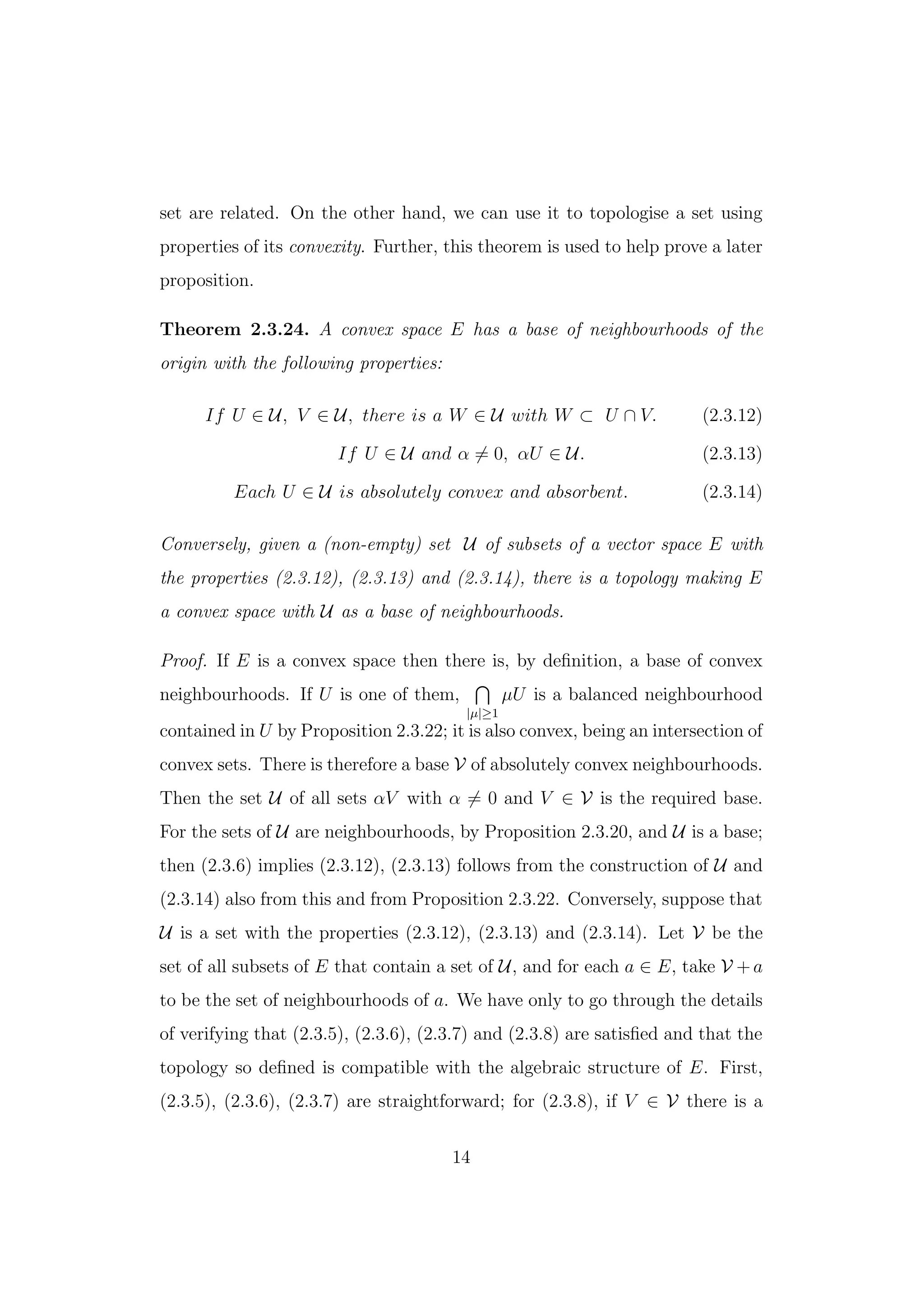
![U ∈ U with U ⊂ V and then it is easy to show that V +a is a neighbourhood
of every point of 1
2
U +a. To prove the continuity of addition at x = a, y = b,
let U ∈ U; then if x ∈ 1
2
U + a and y ∈ 1
2
U + b, x + y ∈ U + a + b. Finally,
to prove that λx is continuous at λ = α, x = a, it is enough to find η and
δ so that λx − αa ∈ U whenever |λ − α| < η and x ∈ δU + a. Now there
is a µ > 0 with a ∈ µU; choose η so that 0 < 2η < µ−1
and then δ so that
0 < 2δ < (|α| + η)−1
. Then
λx − αa = λ(x − a) + (λ − α)a ∈ (|α| + η)δU + ηµU ⊂ U.
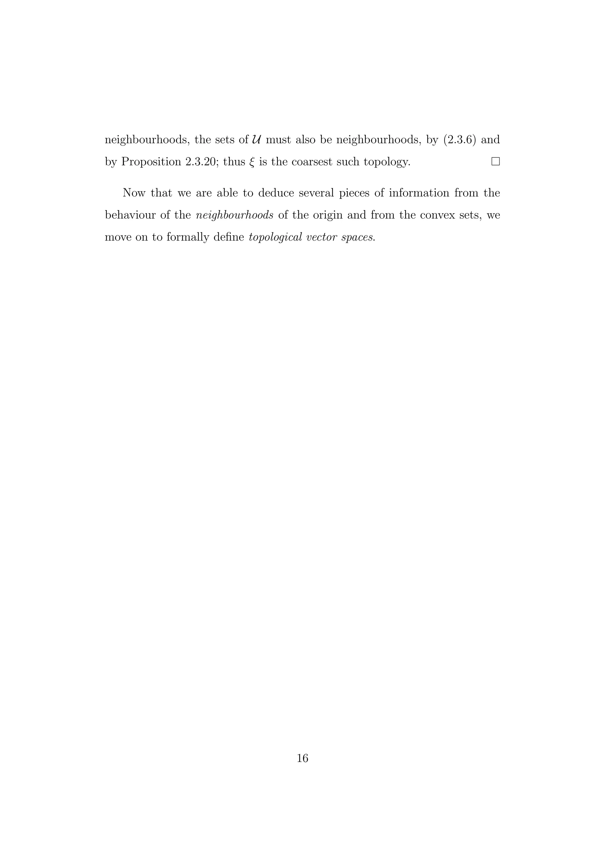
The above theorem has a useful corollary, which we shall now state and
prove. The formulation of the corollary and its proof is taken from [5][page
11].
Corollary 2.3.25. Let V be any set of absolutely convex absorbent subsets
of a vector space E. Then there is a coarsest topology on E compatible with
the algebraic structure in which every set in V is a neighbourhood. Under
this topology E is convex and a base of neighbourhoods is formed by the sets
1≤i≤n
Vi,
where > 0, Vi ∈ V.
Proof. The set U of subsets of the form
1≤i≤n
Vi,
where > 0, Vi ∈ V satisfies the conditions (2.3.12), (2.3.13) and (2.3.14)
and so U is a base of neighbourhoods in a topology ξ on E making E a
convex space. Also in any compatible topology in which the sets of V are
15](https://image.slidesharecdn.com/83ed9392-09ad-4275-b5fe-da6bc7d962f4-150716125805-lva1-app6891/75/Topological_Vector_Spaces_FINAL_DRAFT-16-2048.jpg)
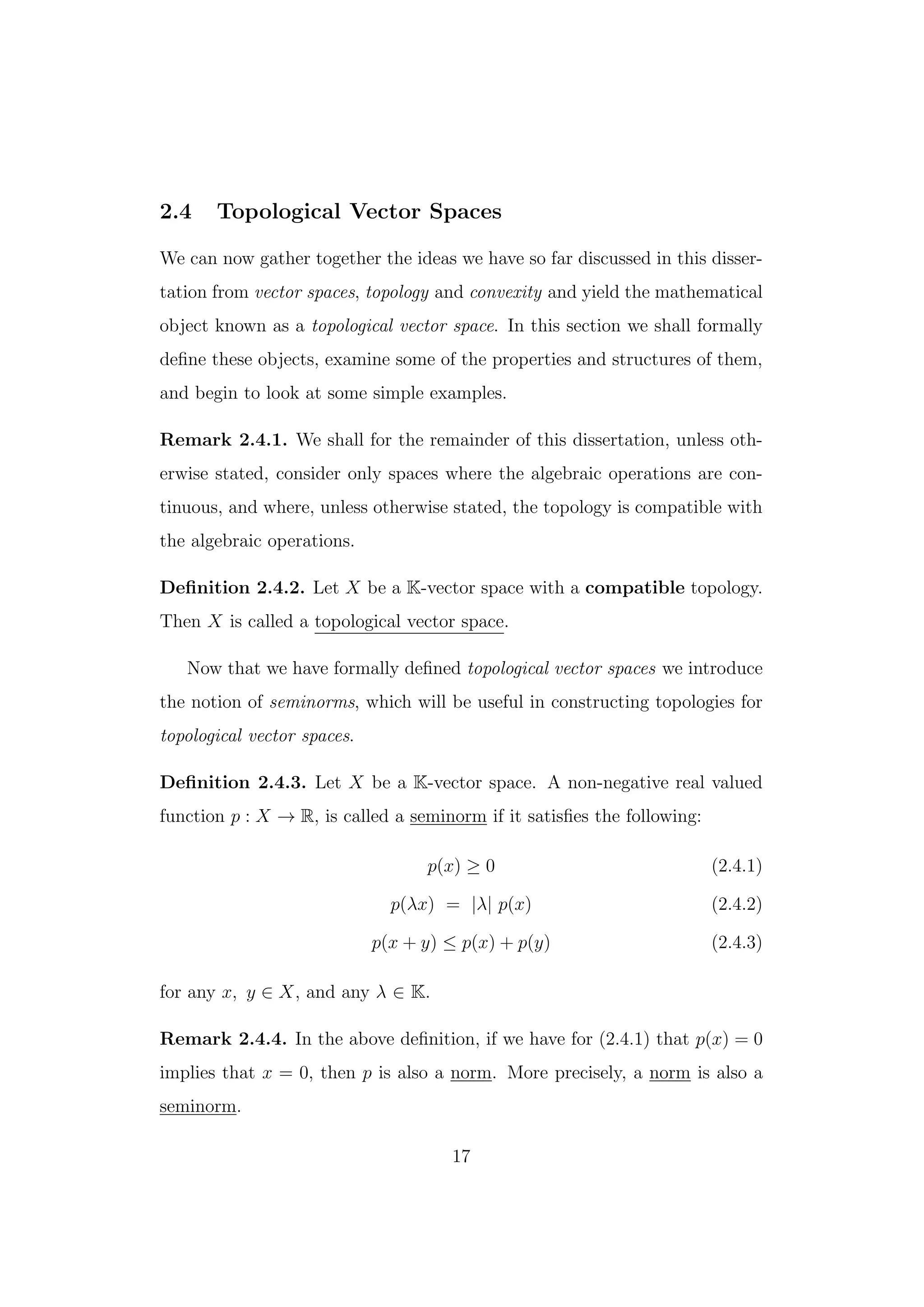
![Definition 2.4.5. Let X be a K-vector space. X is called a seminormed space
if there exists on X a seminorm. X is called a normed space if a norm is de-
fined on X. If a normed space is also complete, i.e.: every Cauchy sequence
of points in X converges in X, X is called a Banach space.
Before continuing, we now show two simple examples demonstrating how
a space can be topologised using convexity and using norms. The two exam-
ples below are taken from [5][Chapter 1 Supplement].
Example 2.4.6. We take a Euclidean n-dimensional space X, where as
usual, an element x ∈ X denotes the point x = (x1, x2, ..., xn). X becomes a
convex space under the topology induced by the norm
x =
1≤i≤n
|xi|2
. (2.4.4)
In this case, we find that this topology is in fact the only compatible topology
with the algebraic structure of the finite-dimensional space.
Example 2.4.7. Let C be the set of all real valued functions which, on a
bounded closed interval [a, b], are continuous. Then C becomes convex under
the supremum norm
f = sup
a≤l≤b
|f(l)|, (2.4.5)
where f(l) denotes the value of the function f at the point l.
Remark 2.4.8. In Example 2.4.7 above, the case of complex valued functions
is analogous.
We now move on to look at how the relationship between seminorms
and neighbourhoods can be used to tell us about the structure of the entire
space that we are concerned with. For the remainder of this section we have
18](https://image.slidesharecdn.com/83ed9392-09ad-4275-b5fe-da6bc7d962f4-150716125805-lva1-app6891/75/Topological_Vector_Spaces_FINAL_DRAFT-19-2048.jpg)
![used material from [5] which focusses on seminorms. Where more details or
context may be desired, we specify the location of the source material.
The following proposition can be found in [5][page 13], and tells us that
there is a connection between seminorms and absolutely convex absorbent
sets. Its proof is from the same source, although we expand slightly on some
details.
Proposition 2.4.9. Let p be a seminorm on a K-vector space E. Then for
each α > 0, λ ∈ K, the sets
{x ∈ X p(x) < λ}
and
{x ∈ X p(x) ≤ λ}
are absolutely convex and absorbent.
To each absolutely convex absorbent subset A of E corresponds a seminorm
p, defined by
p(x) = inf λ λ > 0, x ∈ λA ,
and with the property that
x p(x) < 1 ⊂ A ⊂ x p(x) ≤ 1 .
Proof. This immediately follows from the finiteness of p, and from (2.4.2)
and (2.4.3). In the case of (2.4.2) it clearly holds that p(x) < λ and p(x) ≤ λ
hold, since we have p(λx) = |λ|p(x), which implies that p(x) < λ
|λ|
= 1 and
p(x) ≤ λ
|λ|
= 1 which are absolutely convex and absorbent. As for (2.4.3),
take p(x + y) < λ and p(x + y) ≤ λ. Then p(x + y) ≤ p(x) + p(y) < λ
and p(x + y) ≤ p(x) + p(y) ≤ λ clearly hold since p(x) < λ, p(y) < λ and
p(y) ≤ λ respectively. Since p is a seminorm, and E is a vector space and
19](https://image.slidesharecdn.com/83ed9392-09ad-4275-b5fe-da6bc7d962f4-150716125805-lva1-app6891/75/Topological_Vector_Spaces_FINAL_DRAFT-20-2048.jpg)
![hence is convex, and so we have that the properties hold.
For the second part, the fact that A is absorbent ensures that p(x) is finite
for each x ∈ E. The conditions (2.4.1) and (2.4.2) are clearly satisfied; for
(2.4.3), let x ∈ λA and y ∈ µA with λ > 0, µ > 0. Then
x + y ∈ λA + µA = (λ + µ)A
and so
p(x + y) ≤ λ + µ.
Hence, p(x + y) ≤ p(x) + p(y). The last part follows from the definition of
p.
The above proposition gives rise to a notion which can be very useful
when working with seminorms.
Definition 2.4.10. The seminorm p corresponding to the absolutely con-
vex set A as in Proposition 2.4.9 is known as the gauge of A.
We now give some properties of gauges before continuing with examples
concerning seminorms. These properties are taken from [5][page 14].
Properties 2.4.11. Let p be a gauge of the absolutely convex absorbent
set A as in Proposition 2.4.9. If q is also the gauge of the absolutely convex
absorbent set B, the we have the following:
If λ = 0, the gauge of λA is |λ|−1
p. (2.4.6)
The gauge of A ∩ B is sup{p, q}. (2.4.7)
If A ⊂ B then q(x) ≤ p(x) for all x ∈ X. (2.4.8)
Also of interest is the following statement, also from [5, page 14].
20](https://image.slidesharecdn.com/83ed9392-09ad-4275-b5fe-da6bc7d962f4-150716125805-lva1-app6891/75/Topological_Vector_Spaces_FINAL_DRAFT-21-2048.jpg)
![Statement 2.4.12. If p is the gauge of A, it is also the gauge of every
absolutely convex absorbent set B which satisfies
{x p(x) < 1} ⊂ B ⊂ {x p(x) ≤ 1}.
Proof. The proof of Statement 2.4.12 uses the same arguement as the proof
of Proposition 2.4.9, relating most heavily to the latter part of the proof.
We now state and prove a proposition found in [5][page 14], regarding
continuity of seminorms. With this we will have a lot of tools at our disposal
for understanding the topology of many spaces. We first must define an
interior however. We again use [5] [page 6], simply for consistency.
Definition 2.4.13. A point x is called an interior point of the subset A of
E if there is a neighbourhood U of x contained in A. The set of all interior
points of A is an open set contained in A called the interior (of A).
Proposition 2.4.14. In a convex space E, a seminorm p is continuous if
and only if it is continuous at the origin.
If p is the gauge of the absolutely convex absorbent set U, p is continuous if
and only if U is a neighbourhood. In this case the interior of U is given by
{x p(x) < 1}.
Proof. If p is continuous at the origin and > 0 is given, there is a neigh-
bourhood V with p(x) < for x ∈ V . Now, if a is any point of E,
|p(x) − p(a)| ≤ p(x − a) < for x ∈ a + V .
For the second part, if U is a neighbourhood and > 0 is given, then p(x) ≤
for x ∈ U and so p is continuous at the origin, and by i), on E also. If p
is continuous then V = {x|p(x) < 1} is open, being the inverse image of
the open interval (−∞, −1) ∪ (1, ∞). But V ⊂ U and so U is a neighbour-
hood.
21](https://image.slidesharecdn.com/83ed9392-09ad-4275-b5fe-da6bc7d962f4-150716125805-lva1-app6891/75/Topological_Vector_Spaces_FINAL_DRAFT-22-2048.jpg)
![So we clearly see that there is some connection between seminorms and
absolutely convex absorbent sets. This implies that we can describe the
topology of a convex space using seminorms. The following is a common way
of creating a convex space topology. This particular formulation and its proof
below can be seen in [5, pages 10- 15].
Theorem 2.4.15. Given any set Q of seminorms on a vector space X, there
is a coarsest topology on X compatible with the algebraic structure in which
every seminorm in Q is continuous, i.e.:continuous at the origin. Under this
topology, X is a convex space and a base of closed neighbourhoods is formed
by the sets
{x sup
1≤i≤n
pi(x) ≤ },
where > 0 and pi ∈ Q.
Proof. This follows from Corollary 2.3.25 and from Proposition 2.4.14. For
if pi is the gauge of the absolutely convex neighbourhood Vi, then −1
sup
1≤i≤n
pi
is the gauge of
1≤i≤n
Vi.
Remark 2.4.16. When using the term convex space, it is to emphasise that
the set is made convex by the topology rather than simply being a result of
it being a vector space. Of course, we are here dealing with vector spaces
which are convex by definition. We are however highlighting the fact that
we can make sets convex using topologies and neighbourhoods which induce
topologies, and thus convexity.
In summary, we have discussed how we can topologise a set using convex-
ity and (families of) convex subsets, and by using (families of) seminorms.
Furthermore, one of the most fundamental and powerful results discussed is
that behaviour at the origin determines the behaviour everywhere, mainly
as we can translate any neighbourhood of the origin to any other part of the
22](https://image.slidesharecdn.com/83ed9392-09ad-4275-b5fe-da6bc7d962f4-150716125805-lva1-app6891/75/Topological_Vector_Spaces_FINAL_DRAFT-23-2048.jpg)
![space we are interested in working in. Furthermore, for any topological vector
space, any open neighbourhood of the origin is absorbing and contains a bal-
anced neighbourhood[4]. In the next section, we will look at a few examples
and apply what we have done so far.
23](https://image.slidesharecdn.com/83ed9392-09ad-4275-b5fe-da6bc7d962f4-150716125805-lva1-app6891/75/Topological_Vector_Spaces_FINAL_DRAFT-24-2048.jpg)
![3 Examples and applications
In this section of the dissertation we focus on applying the theory discussed
in the first section to simple examples. There will be very few definitions, as
they will only be given if necessary to contextualise an example.
3.1 Normed Spaces
We start with a simple example, where we can clearly see that we have a
compatible topology which is induced by a norm. A copy of this example can
be found in [3][page 9].
Example 3.1.1. Let X = Rn
be a vector space and let a norm defined on
X be given by
x p :=
n
j=1
|xj|p
1
p
,
where 1 ≤ p < ∞. Clearly this satisfies the properties of seminorms (any
norm is itself a seminorm) and simply by inspection we can see that a con-
vexity is induced by the topology of this norm. Furthermore, it is easy to
find subsets that are absolutely convex and absorbent, through which we can
describe the topology.
3.2 Metric spaces, and the space p
For our next examples, we assume knowledge of metrics, convergence and
sequences. We need to introduce the space p for our next example. This
particular formulation is taken from [3][page 12].
24](https://image.slidesharecdn.com/83ed9392-09ad-4275-b5fe-da6bc7d962f4-150716125805-lva1-app6891/75/Topological_Vector_Spaces_FINAL_DRAFT-25-2048.jpg)
![Definition 3.2.1. Let 1 ≤ p < ∞. We define p(K) to consist of all sequences
(ak)k∈N, ak ∈ K, such that
(ak)k∈N p :=
∞
k=1
|ak|p
1
p
< ∞.
Remark 3.2.2. The space p can be used to derive and prove Minkowski’s
Inequality. We can further obtain and prove H¨older’s Inequality and Jensen’s
Inequality. We shall not do this here, but we observe this since these are
powerful results in functional analysis.
Example 3.2.3. Let X be set on which the ∞ norm is defined. We then
find that X is in fact a Banach space. Therefore it is Hausdorff and locally
convex.
The following definition and example are taken from [10].
Definition 3.2.4. Let X be a metrisable set. If X is (locally) convex and
complete, then X is a Fr´echet space. Its topology is defined by a countable
family of seminorms.
Example 3.2.5. Let X be the space of smooth functions on [0, 1]. Then
X is a Fr´echet space. We take its topology as the C∞
topology (infinitely
differentiable functions) which is given by the countable family of seminorms
f α = sup |Dα
f|,
and since fn → f in this topology, it implies that f is smooth, i.e.:
Dα
fn → Dα
f,
and so any Cauchy sequence has a limit in the space of smooth functions,
and thus X is complete.
25](https://image.slidesharecdn.com/83ed9392-09ad-4275-b5fe-da6bc7d962f4-150716125805-lva1-app6891/75/Topological_Vector_Spaces_FINAL_DRAFT-26-2048.jpg)
![4 Further Reading
There is an extensive range of literature available concerning the theory of
topological vector spaces, certain types of spaces such as Banach and Hilbert
spaces and more generally there is an abundance of material available on
functional analysis. Furthermore there is a vast range of writing available on
topology and its many applications, many of which are beyond the scope of
this dissertation. The consolidation of ideas within topology and functional
analysis themselves have far reaching consequences in many other areas of
mathematics. We have in this project focussed our attention on only a few
manners in which they interact. The sources used to produce this dissertation
go in to much greater detail than we have done so here, and would provide
much deeper explanation of the material, as well as stretching to much further
and deeper applications of the concepts discussed, and some we have not.
References
[1] Bourbaki. N, Elements of the history of mathematics. Electronic copy
of book online. Springer, 1994. Accessed 18/03/2015 https://books.
google.co.uk/books?id=Qvo8-KC__VAC&pg=PA207&lpg=PA207&dq=
history+of+topological+vector+spaces&source=bl&ots=
Lu56iuEr2H&sig=6AUc4twV8kMjgrz47FHAYN9WFdM&hl=en&sa=X&ei=
KrwJVdenB8StU5KqhLgC&ved=0CFIQ6AEwCA#v=onepage&q&f=false
[2] Crossley. M, Essential Topology, Springer Undergraduate Mathematics
Series, 2005.
[3] Jacob. N, Functional Analysis I + II: I Banach and Hilbert Spaces, II
Linear Operators, Lecture Notes, Swansea University.
26](https://image.slidesharecdn.com/83ed9392-09ad-4275-b5fe-da6bc7d962f4-150716125805-lva1-app6891/75/Topological_Vector_Spaces_FINAL_DRAFT-27-2048.jpg)
![[4] Kupferman. R, Topological Vector Spaces, Lecture Notes, The Hebrew
University of Jerusalem. Used between October 2014 and March 2015.
[5] Robertson. A.P and Robertson. W, Topological Vector Spaces, Cam-
bridge University Press, 1973.
[6] Wallace. A.H, Differential Topology First Steps, University of Pennsyl-
vania, 1968.
[7] Wong. Y, Introductory Theory of Topological Vector Spaces, Mono-
graphs and textbooks in pure and applied mathematics, 1992.
[8] Figure 1, convex set http://mathworld.wolfram.com/Convex.html,
visited on 16/03/2015.
[9] Open map definition http://mathworld.wolfram.com/OpenMap.html,
visited on 16/03/2015.
[10] Fr´echet Space, definition and example http://mathworld.wolfram.
com/FrechetSpace.html, visited on 17/03/15.
27](https://image.slidesharecdn.com/83ed9392-09ad-4275-b5fe-da6bc7d962f4-150716125805-lva1-app6891/75/Topological_Vector_Spaces_FINAL_DRAFT-28-2048.jpg)