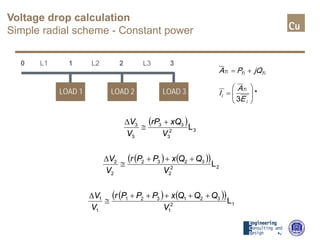
Angelo Baggini, angelo.baggini@unibg.it, Bergamo University - Engineering Department
Via Marconi 5, 24044 Dalmine (BG) – Italy
Voltage drop calculation in cable lines
1. Data required to start
A. Cable parameters
B. Load characteristics
C. Distribution Scheme
D. Maximum voltage drop
2. Voltage drop calculation
in case of:
A. Radial line
1. constant current
2. constant power
B. Shunted line
C. Long line
Voltage drop calculation in cable lines
Data required to start
1. Cable parameters (affecting voltage drop)
• R Resistance
• X Reactance
• C Capacitance
• G Conducance
2. Load characteristics
• Impedance
• Power
• Current
3. Installation characteristics
• System type, rated frequency and voltage
• Line length (L)
• Type of distribution
4. Maximum allowed voltage drop
• technical standards
• proper working conditions of loads
• steady state conditions - transient conditions
Voltage drop calculation in cable lines
Data required to start
Cable parameters
A
Data required to start
Cable parameters
R L
Data required to start
Cable parameters
R L
C
Data required to start
Cable parameters
R L
C G
Data required to start
Cable parameters – Long lines
R L
C
R L
C G
R L
R L
C
R L
C G
R L
R L
R L
C G
R L
…
…
…
Data required to start
Cable parameters
R L
C
R L
C G
R L
Data required to start
Cable parameters
R
𝑅𝑅 = ρ(θ)
1
𝑆𝑆
(Ω/m)
𝐿𝐿 =
µ
2π
𝑙𝑙𝑙𝑙
2𝐷𝐷
𝑑𝑑
(H/m)
L
D
d
Data required to start
Cable parameters
G
C 𝐶𝐶 =
2πε
𝑙𝑙 𝑙𝑙
2𝐷𝐷
𝑑𝑑
(F/m)
D
d
T(r)=90°C
Data required to start
LV Cable parameters
Rated
section
(mm2)
d.c.
(Ohm/km)
a.c.
(Ohm/km)
d.c.
(Ohm/km)
a.c.
(Ohm/km)
Flexible
conductor
Flexible
conductor
Rigid
conductor
Rigid
conductor
1.5 16.95 16.95 15.4 15.4
2.5 10.17 10.17 9.45 9.45
4 6.31 6.31 5.88 5.88
6 4.20 4.20 3.93 3.93
10 2.43 2.43 2.33 2.33
16 1.54 1.54 1.47 1.47
25 0.99 0.99 0.93 0.93
F=50 Hz
Data required to start
LV Cable parameters
Rated
section
(mm2)
Unipolar
(Ohm/km)
Multipolar
(Ohm/km)
Unipolar
(Ohm/km)
Multipolar
(Ohm/km)
G-SETTE G-SETTE G-SETTE + G-SETTE +
1.5 0.146 0.103 0.144 0.100
2.5 0.135 0.095 0.132 0.094
4 0.126 0.090 0.122 0.087
6 0.118 0.085 0.144 0.083
10 0.106 0.079 0.105 0.078
16 0.099 0.076 0.098 0.075
25 0.095 0.075 0.093 0.074
Elastomeric insulation
(Data required to start)
Service reactance
Theoretically only for …
Practically …
R L M
33323213133
323222121222
31321211111
ILjIMjIMjIRE
IMjILjIMjIRE
IMjIMjILjIRE
⋅+⋅+⋅+⋅=
⋅+⋅+⋅+⋅=
⋅+⋅+⋅+⋅=
ωωω
ωωω
ωωω ( )( )
( )( )
( )( ) 3333
2
33
22
2
2222
111
2
111
IMLjRILjIMjIMjIRE
IMLjRIMjILjIMjIRE
IMLjRIMjIMjILjIRE
SSSSS
SSSSS
SSSSS
⋅−+=⋅+⋅⋅+⋅⋅+⋅=
⋅−+=⋅⋅+⋅+⋅⋅+⋅=
⋅−+=⋅⋅+⋅⋅+⋅+⋅=
ωωαωαω
ωαωωαω
ωαωαωω
SMLL S −=
MV cable resitance
(50 Hz – 90 °C)
Source Prismyan catalogue 2014
MV cable reactance
(50 Hz – 90 °C)
Source Prismyan catalogue 2014
MV cable reactance
(50 Hz – 90 °C)
Source Prismyan catalogue 2014
MV cable reactance
(50 Hz – 90 °C)
Source Prismyan catalogue 2014
MV HEPR cable capacitance
Source Prismyan catalogue 2014
Voltage drop calculation in cable lines
Data required to start
Load type
B
Load type
Costant impendance
Constant power
… statistically also the ones at costant impedance became at constant power
… sometime loads are considered having a constant current
Z
Voltage drop calculation in cable lines
Data required to start
Installation characteristics
C
Distribution scheme
Simple radial
Shunted
Rated frequency and voltage
LOAD
LOAD 3LOAD 2LOAD 1
L
L3L2L1
Voltage drop calculation in cable lines
Data required to start
Maximum allowed voltage drop
D
Data required to start
Maximum allowed voltage drop
Technical standards
• LV Utilization: IEC 60364
• 4% general loads
• 5% lighting
Proper working conditions of loads
• Steady state conditions
• 2% ?
• Transient conditions
• 10% ?
(indirect reference to EN 50160)
Voltage drop calculation in cable lines
Simple radial scheme
Constant current
Voltage drop calculation
Simple radial scheme - Constant current
AC
DC
RAC L
RAC L
RDC
Voltage drop calculation
Simple radial scheme - Constant current
AC
∆V = K L I (RAC cosϕ + X sinϕ) < ∆VM
K = 2 for single-phase lines
K = √(3) for tree-phase lines
DC
∆V = 2 L I RDC
• Cable R and X
• Line length (L)
• Load Current I (standard)
• Phase displacement (ϕ) (standard)
Load
I=50 A, 400 V 3 phase
Installation
T=40 °C
L=100 m
Maximum Voltage drop
steady-state 2%
inrush 10%
Cable Type
3 conductors – EPR
Voltage drop calculation
Simple radial scheme - Constant current
T(r)=90°C
Voltage drop calculation
Simple radial scheme - Constant current
Rated
section
(mm2)
d.c.
(Ohm/km)
a.c.
(Ohm/km)
d.c.
(Ohm/km)
a.c.
(Ohm/km)
Flexible
conductor
Flexible
conductor
Rigid
conductor
Rigid
conductor
1.5 16.95 16.95 15.4 15.4
2.5 10.17 10.17 9.45 9.45
4 6.31 6.31 5.88 5.88
6 4.20 4.20 3.93 3.93
10 2.43 2.43 2.33 2.33
16 1.54 1.54 1.47 1.47
25 0.99 0.99 0.93 0.93
F=50 Hz
Voltage drop calculation
Simple radial scheme - Constant current
Rated
section
(mm2)
Unipolar
(Ohm/km)
Multipolar
(Ohm/km)
Unipolar
(Ohm/km)
Multipolar
(Ohm/km)
G-SETTE G-SETTE G-SETTE + G-SETTE +
1.5 0.146 0.103 0.144 0.100
2.5 0.135 0.095 0.132 0.094
4 0.126 0.090 0.122 0.087
6 0.118 0.085 0.144 0.083
10 0.106 0.079 0.105 0.078
16 0.099 0.076 0.098 0.075
25 0.095 0.075 0.093 0.074
Elastomeric insulation
Voltage drop calculation
Simple radial scheme - Constant current
∆V(S) = K L I (R cosϕ + X sinϕ) < ∆VM
∆V(6) = 29,52 V
∆V% = ∆V/V = 13,54% > 2%
K = √(3)
R(6)= 4,20 (ohm/km)
X(6)=0.083 (ohm/km)
L=100 m
cosϕ =0.8
Voltage drop calculation
Simple radial scheme - Constant current
∆V(S) = K L I (R cosϕ + X sinϕ) < ∆VM
S= 6 mm2  ∆V% = 13,4% > 2%
S=10 mm2  ∆V% = 4.3 % >2%
S=16 mm2  ∆V% = 2.7% > 2%
S=25 mm2  ∆V% = 1.8%< 2% ∆V(25)= 7.25 V
K = √(3)
R(10)= 2.430 (ohm/km)
X(10)=0.078 (ohm/km)
L=100 m
cosϕ =0.8
Voltage drop calculation
Simple radial scheme - Constant current
RAC L RLOAD LLOADI
E = ((RAC+RLOAD)+j (LAC+LLOAD)) I
LOAD
Voltage drop calculation in cable lines
Simple radial scheme
Constant power
Voltage drop calculation
Simple radial scheme - Constant power
111 jQPA +=LOAD
*
3 1
1
1 





=
E
A
I
V0
0 1
R jX
LOADV0
E0
LOAD
R jX
V1
E1
Voltage drop calculation
Simple radial scheme - Constant power
L
3
)()(
3
jQ-P
)(
1
1111
1
11
⋅
+−++
=⋅⋅+=∆
E
xPrQjxQrP
E
LjxrE
111 jQPA +=
3E
jQ-P
*
3 1
11
1
1
1 =





=
E
A
I
E0
LOAD
R jX
E1
Voltage drop calculation
Simple radial scheme - Constant power
( ) ( )
33
1
2
2
1
11
2
2
1
11
10 




 +−
+




 +
+= L
E
xPrQ
L
E
xQrP
EE
L
3
)(
L
3
)(
1
11
1
11
10 ⋅
+−
+⋅
+
=−=∆
E
xPrQ
j
E
xQrP
EEE
L
3
)(
L
3
)(
1
11
1
11
10 ⋅
+−
+⋅
+
+=
E
xPrQ
j
E
xQrP
EE
0E
1E L
3
)(
1
11
⋅
+
E
xQrP
L
3
)(
1
11
⋅
+−
E
xPrQ
j
Voltage drop calculation
Simple radial scheme - Constant power
( ) ( ) ( )
( )L
E
xQrP
E
E
xQrP
EL
E
xQrP
EL
E
xQrP
EE
3
L
33
1
3
1
11
1
11
12
1
11
1
2
1
11
10
+
≅∆
+
+=




 +
+=




 +
+≅�
111 jQPA +=
3E
jQ-P
*
3 1
11
1
1
1 =





=
E
A
I
E0
LOAD
R jX
E1
Voltage drop calculation
Simple radial scheme - Constant power
( )L
E
xQrP
E
3 1
11 +
≅∆
111 jQPA +=
3E
jQ-P
*
3 1
11
1
1
1 =





=
E
A
I
E0
LOAD
R jX
E1
( ) ( )
3 2
1
11
2
1
11
L
V
xQrP
L
E
xQrP
E
E
V
V +
=
+
≅
∆
=
∆
Voltage drop calculation
Simple radial scheme - Constant power
BUT
E1 is the voltage at the end of the line while usually we
know the voltage at the begin of the line!
( )L
E
xQrP
E
3 1
11 +
≅∆
111 jQPA +=
3E
jQ-P
*
3 1
11
1
1
1 =





=
E
A
I
E0
LOAD
R jX
E1
Load
P=6 MW
Q=4,5 Mvar,
20 kV 3 phase
Installation
T=20 °C
L= 5 km
Cable Type
1X – XLPE
Voltage drop calculation
Simple radial scheme - Constant power
Voltage drop calculation
Simple radial scheme - Constant power
Parameter Value
I (A) – approximated - 216,5
Section (mm2) 70
Capacity (A) 255
r (Ω/km) 0,346
x (Ω/km) 0,131
Voltage drop calculation
Simple radial scheme - Constant power
Iteration (k) ∆V (V) V1 (V)
0 666,375 19333,63
1 689,343 19310,66
2 690,162 19309,84
3 690,192 19309,81
( )L
V
xQrP
V
1
11 +
≅∆
( )L
E
xQrP
E
3 1
11 +
≅∆
)(
0
)1(
1
kk
VVV ∆−=+
Voltage drop calculation in cable lines
Shunted scheme
Constant power
Voltage drop calculation
Simple radial scheme - Constant power
• Neglecting P and Q of fed lines (i+…)
• Same section for the entire line
( )
i
i
TiTi
i L
E
xQrP
E
3
1
+
≅∆ −
TiTiTi jQPA +=
*
3 





=
i
Ti
i
E
A
I
L3L2L1
LOAD 3LOAD 2LOAD 1
0 1 2 3
Voltage drop calculation
Simple radial scheme - Constant power
TiTiTi jQPA +=
*
3 





=
i
Ti
i
E
A
I
L3L2L1
LOAD 3LOAD 2LOAD 1
0 1 2 3
( )
( ) ( )( )
( ) ( )( )L
L
L
12
1
321321
1
1
22
2
3232
2
2
32
3
33
3
3
V
QQQxPPPr
V
V
V
QQxPPr
V
V
V
xQrP
V
V
+++++
≅
∆
+++
≅
∆
+
≅
∆
Voltage drop calculation
Simple radial scheme - Constant power
TiTiTi jQPA +=
*
3 





=
i
Ti
i
E
A
I
L3L2L1
LOAD 3LOAD 2LOAD 1
0 1 2 3
V V Vi
k
i i
k( ) ( )+
−= −1
1 ∆ V V Vi
k
i
k
i
k( ) ( ) ( )+
= −1
∆
( ) ( )( )
( ) ( )( )
)1(
10
)1(
1
1
1
321321)1(
1
)0(
10
)0(
1
1
0
321321)0(
1
VVV
L
V
QQQxPPPr
V
VVV
L
V
QQQxPPPr
V
∆−=
+++++
≅∆
∆−=
+++++
≅∆
Voltage drop calculation
Simple radial scheme - Constant power
L3L2L1
LOAD 3LOAD 2LOAD 1
0 1 2 3
1. Selection of the section according with
• current rating (L1)
• Total approx voltage drop
2. Voltage drop calculation on each line
segment (iterated)
3. Current calculation (iterated)
*
3 





=
i
Ti
i
E
A
I
( )∆V
rP xQ
V
i
Ti Ii
i≅
+
0

( )
x+
1 N
1=i10
0
01
0
1
0






−=
+
−≅∆−=
∑∑
∑∑
=
==
iTiiTi
N
i
i
TiTi
N
i
i
N
i
N
LQLPr
V
V
L
V
xQrP
VVVV
�
Voltage drop calculation
Simple radial scheme - Constant power
L3L2L1
LOAD 3LOAD 2LOAD 1
0 1 2 3
Parameter
Node
0 1 2 3 4
V (kV) 20 ? ? ? >19
L (km) -- 6 0,4 1 0,2
P (MW) -- 2,3 3 1 1
Q (Mvar) -- 1 2 0,5 0,5
L4
LOAD 4
4
Ref. Conductor temperature 90 °C
AIR
Voltage drop calculation
Simple radial scheme - Constant power
Selection of the section - current rating
L3L2L1
LOAD 3LOAD 2LOAD 1
0 1 2 3 L4
LOAD 4
4
A
E
A
I
T
29,240
3
*
0
0
0 =





=
Parameter
Node
0 1 2 3 4
V (kV) 20 ? ? ? ?
L (km) -- 6 0,4 1 0,2
P (MW) -- 2,3 3 1 1
Q (Mvar) -- 1 2 0,5 0,5
PT (MW) 7,3 7,3 5 2 1
QT (Mvar) 4 4 3 1 0,5
MV cable current capacity
(RG7H1M1 Cu 1X)
Source Prismyan catalogue 2014
AIR
Voltage drop calculation
Simple radial scheme - Constant power
Selection of the section - current capacity
L3L2L1
LOAD 3LOAD 2LOAD 1
0 1 2 3 L4
LOAD 4
4
A
E
A
I
T
29,240
3
*
0
0
0 =





=
Parameter
Node
0 1 2 3 4
V (kV) 20 ? ? ? ?
Li (km) -- 6 0,4 1 0,2
P (MW) -- 2,3 3 1 1
Q (Mvar) -- 1 2 0,5 0,5
PTi (MW) 7,3 7,3 5 2 1
QTi (Mvar) 4 4 3 1 0,5
50 mm2
MV cable resitance
(50 Hz – 90 °C)
Source Prismyan catalogue 2014
MV cable reactance
(50 Hz – 90 °C)
Source Prismyan catalogue 2014
Voltage drop calculation
Simple radial scheme - Constant power
Selection of the section – Voltage drop
L3L2L1
LOAD 3LOAD 2LOAD 1
0 1 2 3 L4
LOAD 4
4
18,607kVx+
1 4
1=i
4
10
04 =





−= ∑∑=
iTi
i
iTi LQLPr
V
VV
Parameter
Node
0 1 2 3 4
V (kV) 20 ? ? ? ?
Li (km) -- 6 0,4 1 0,2
P (MW) -- 2,3 3 1 1
Q (Mvar) -- 1 2 0,5 0,5
PTi (MW) 7,3 7,3 5 2 1
QTi (Mvar) 4 4 3 1 0,5
PTi Li -- 43,800 2,000 2,000 0,200
QTi Li -- 24,000 1,200 1,000 0,100
50mm2
r=0,495
x=0,150
Voltage drop calculation
Simple radial scheme - Constant power
Selection of the section – Voltage drop
L3L2L1
LOAD 3LOAD 2LOAD 1
0 1 2 3 L4
LOAD 4
4
18,990kVx+
1 4
1=i
4
10
04 =





−= ∑∑=
iTi
i
iTi LQLPr
V
VV
Parameter
Node
0 1 2 3 4
V (kV) 20 ? ? ? ?
L (km) -- 6 0,4 1 0,2
P (MW) -- 2,3 3 1 1
Q (Mvar) -- 1 2 0,5 0,5
PTi (MW) 7,3 7,3 5 2 1
QTi (Mvar) 4 4 3 1 0,5
PTi Li -- 43,800 2,000 2,000 0,200
QTi Li -- 24,000 1,200 1,000 0,100
70mm2
r=0,344
x=0,140
Voltage drop calculation
Simple radial scheme - Constant power
Selection of the section – Voltage drop
L3L2L1
LOAD 3LOAD 2LOAD 1
0 1 2 3 L4
LOAD 4
4
19,233kVx+
1 4
1=i
4
10
04 =





−= ∑∑=
iTi
i
iTi LQLPr
V
VV
Parameter
Node
0 1 2 3 4
V (kV) 20 ? ? ? ?
L (km) -- 6 0,4 1 0,2
P (MW) -- 2,3 3 1 1
Q (Mvar) -- 1 2 0,5 0,5
PTi (MW) 7,3 7,3 5 2 1
QTi (Mvar) 4 4 3 1 0,5
PTi Li -- 43,800 2,000 2,000 0,200
QTi Li -- 24,000 1,200 1,000 0,100
95mm2
r=0,248
x=0,130
Voltage drop calculation
Simple radial scheme - Constant power
Accurated Voltage drop calculation
L3L2L1
LOAD 3LOAD 2LOAD 1
0 1 2 3 L4
LOAD 4
4
Parameter
Node
0 1 2 3 4
PTi Li -- 43,800 2,000 2,000 0,200
QTi Li -- 24,000 1,200 1,000 0,100
r PTi Li + x QTi Li -- 13,9824 0,652 0,626 0,0626
95 mm2
r = 0,248
x = 0,130
( )
i
i
TiTi
i L
V
xQrP
V �
+
≅∆
Voltage drop calculation
Simple radial scheme - Constant power
Accurated Voltage drop calculation
L3L2L1
LOAD 3LOAD 2LOAD 1
0 1 2 3 L4
LOAD 4
4
95 mm2
r = 0,248
x = 0,130
( )
i
i
TiTi
i L
V
xQrP
V �
+
≅∆
)(
0
)1(
1
kk
VVV ∆−=+
Node (i) 0 1 2 3 4
rPTiLi + xQTiLi -- 13,9824 0,652 0,626 0,0626
Iteraction (k) V (kV) DV (kV) V (kV) DV (kV) V (kV) DV (kV) V (kV) DV (kV) V (kV)
0 20 0,699 19,301 0,0338 19,242 0,0325 19,209 0,0033 19,206
1 -- 0,724 19,276 0,0339 19,242 0,0326 19,209 0,0033 19,206
2 -- 0,724 19,276 0,0339 19,242 0,0326 19,209 0,0033 19,206
Voltage drop calculation in cable lines
Long lines
Long lines
< 300 km < 220 kV
R/2 XL/2
XC
R/2 XL/2
Long lines
< 300 km < 220 kV
R/2 XL/2
XC
R/2 XL/2
L/2L/2
LOAD 2«LOAD 1»
0 1 2
Higher is the number of T more accurated is the result
LOAD 2
Long lines
R XL
XC
R XL
Q = k XL I2
Q = XL I2 - k w C V2
SHORT
LONG
Voltage drop calculation in cable lines
1. Data required to start
A. Cable parameters
B. Load characteristics
C. Distribution scheme
D. Maximum voltage drop
2. Voltage drop calculation in case of:
A. Radial line
1. constant current
2. constant power
B. Shunted line
C. Long line
Thank you
| Presentation title and date
For more information please contact
Angelo Baggini
Università di Bergamo
Dipartimento di Ingegneria
Viale Marconi 5,
24044 Dalmine (BG) Italy
email: angelo.baggini@unibg.it
ECD Engineering Consulting and Design
Via Maffi 21 27100 PAVIA Italy

Power cable - Voltage drop

  • 1.
    Angelo Baggini, angelo.baggini@unibg.it,Bergamo University - Engineering Department Via Marconi 5, 24044 Dalmine (BG) – Italy Voltage drop calculation in cable lines
  • 2.
    Voltage drop calculationin cable lines 1. Data required to start A. Cable parameters B. Load characteristics C. Distribution Scheme D. Maximum voltage drop 2. Voltage drop calculation in case of: A. Radial line 1. constant current 2. constant power B. Shunted line C. Long line
  • 3.
    Voltage drop calculationin cable lines Data required to start
  • 4.
    Data required tostart 1. Cable parameters (affecting voltage drop) • R Resistance • X Reactance • C Capacitance • G Conducance 2. Load characteristics • Impedance • Power • Current 3. Installation characteristics • System type, rated frequency and voltage • Line length (L) • Type of distribution 4. Maximum allowed voltage drop • technical standards • proper working conditions of loads • steady state conditions - transient conditions
  • 5.
    Voltage drop calculationin cable lines Data required to start Cable parameters A
  • 6.
    Data required tostart Cable parameters R L
  • 7.
    Data required tostart Cable parameters R L C
  • 8.
    Data required tostart Cable parameters R L C G
  • 9.
    Data required tostart Cable parameters – Long lines R L C R L C G R L R L C R L C G R L R L R L C G R L … … …
  • 10.
    Data required tostart Cable parameters R L C R L C G R L
  • 11.
    Data required tostart Cable parameters R 𝑅𝑅 = ρ(θ) 1 𝑆𝑆 (Ω/m) 𝐿𝐿 = µ 2π 𝑙𝑙𝑙𝑙 2𝐷𝐷 𝑑𝑑 (H/m) L D d
  • 12.
    Data required tostart Cable parameters G C 𝐶𝐶 = 2πε 𝑙𝑙 𝑙𝑙 2𝐷𝐷 𝑑𝑑 (F/m) D d
  • 13.
    T(r)=90°C Data required tostart LV Cable parameters Rated section (mm2) d.c. (Ohm/km) a.c. (Ohm/km) d.c. (Ohm/km) a.c. (Ohm/km) Flexible conductor Flexible conductor Rigid conductor Rigid conductor 1.5 16.95 16.95 15.4 15.4 2.5 10.17 10.17 9.45 9.45 4 6.31 6.31 5.88 5.88 6 4.20 4.20 3.93 3.93 10 2.43 2.43 2.33 2.33 16 1.54 1.54 1.47 1.47 25 0.99 0.99 0.93 0.93
  • 14.
    F=50 Hz Data requiredto start LV Cable parameters Rated section (mm2) Unipolar (Ohm/km) Multipolar (Ohm/km) Unipolar (Ohm/km) Multipolar (Ohm/km) G-SETTE G-SETTE G-SETTE + G-SETTE + 1.5 0.146 0.103 0.144 0.100 2.5 0.135 0.095 0.132 0.094 4 0.126 0.090 0.122 0.087 6 0.118 0.085 0.144 0.083 10 0.106 0.079 0.105 0.078 16 0.099 0.076 0.098 0.075 25 0.095 0.075 0.093 0.074 Elastomeric insulation
  • 15.
    (Data required tostart) Service reactance Theoretically only for … Practically … R L M 33323213133 323222121222 31321211111 ILjIMjIMjIRE IMjILjIMjIRE IMjIMjILjIRE ⋅+⋅+⋅+⋅= ⋅+⋅+⋅+⋅= ⋅+⋅+⋅+⋅= ωωω ωωω ωωω ( )( ) ( )( ) ( )( ) 3333 2 33 22 2 2222 111 2 111 IMLjRILjIMjIMjIRE IMLjRIMjILjIMjIRE IMLjRIMjIMjILjIRE SSSSS SSSSS SSSSS ⋅−+=⋅+⋅⋅+⋅⋅+⋅= ⋅−+=⋅⋅+⋅+⋅⋅+⋅= ⋅−+=⋅⋅+⋅⋅+⋅+⋅= ωωαωαω ωαωωαω ωαωαωω SMLL S −=
  • 16.
    MV cable resitance (50Hz – 90 °C) Source Prismyan catalogue 2014
  • 17.
    MV cable reactance (50Hz – 90 °C) Source Prismyan catalogue 2014
  • 18.
    MV cable reactance (50Hz – 90 °C) Source Prismyan catalogue 2014
  • 19.
    MV cable reactance (50Hz – 90 °C) Source Prismyan catalogue 2014
  • 20.
    MV HEPR cablecapacitance Source Prismyan catalogue 2014
  • 21.
    Voltage drop calculationin cable lines Data required to start Load type B
  • 22.
    Load type Costant impendance Constantpower … statistically also the ones at costant impedance became at constant power … sometime loads are considered having a constant current Z
  • 23.
    Voltage drop calculationin cable lines Data required to start Installation characteristics C
  • 24.
    Distribution scheme Simple radial Shunted Ratedfrequency and voltage LOAD LOAD 3LOAD 2LOAD 1 L L3L2L1
  • 25.
    Voltage drop calculationin cable lines Data required to start Maximum allowed voltage drop D
  • 26.
    Data required tostart Maximum allowed voltage drop Technical standards • LV Utilization: IEC 60364 • 4% general loads • 5% lighting Proper working conditions of loads • Steady state conditions • 2% ? • Transient conditions • 10% ? (indirect reference to EN 50160)
  • 27.
    Voltage drop calculationin cable lines Simple radial scheme Constant current
  • 28.
    Voltage drop calculation Simpleradial scheme - Constant current AC DC RAC L RAC L RDC
  • 29.
    Voltage drop calculation Simpleradial scheme - Constant current AC ∆V = K L I (RAC cosϕ + X sinϕ) < ∆VM K = 2 for single-phase lines K = √(3) for tree-phase lines DC ∆V = 2 L I RDC • Cable R and X • Line length (L) • Load Current I (standard) • Phase displacement (ϕ) (standard)
  • 30.
    Load I=50 A, 400V 3 phase Installation T=40 °C L=100 m Maximum Voltage drop steady-state 2% inrush 10% Cable Type 3 conductors – EPR Voltage drop calculation Simple radial scheme - Constant current
  • 31.
    T(r)=90°C Voltage drop calculation Simpleradial scheme - Constant current Rated section (mm2) d.c. (Ohm/km) a.c. (Ohm/km) d.c. (Ohm/km) a.c. (Ohm/km) Flexible conductor Flexible conductor Rigid conductor Rigid conductor 1.5 16.95 16.95 15.4 15.4 2.5 10.17 10.17 9.45 9.45 4 6.31 6.31 5.88 5.88 6 4.20 4.20 3.93 3.93 10 2.43 2.43 2.33 2.33 16 1.54 1.54 1.47 1.47 25 0.99 0.99 0.93 0.93
  • 32.
    F=50 Hz Voltage dropcalculation Simple radial scheme - Constant current Rated section (mm2) Unipolar (Ohm/km) Multipolar (Ohm/km) Unipolar (Ohm/km) Multipolar (Ohm/km) G-SETTE G-SETTE G-SETTE + G-SETTE + 1.5 0.146 0.103 0.144 0.100 2.5 0.135 0.095 0.132 0.094 4 0.126 0.090 0.122 0.087 6 0.118 0.085 0.144 0.083 10 0.106 0.079 0.105 0.078 16 0.099 0.076 0.098 0.075 25 0.095 0.075 0.093 0.074 Elastomeric insulation
  • 33.
    Voltage drop calculation Simpleradial scheme - Constant current ∆V(S) = K L I (R cosϕ + X sinϕ) < ∆VM ∆V(6) = 29,52 V ∆V% = ∆V/V = 13,54% > 2% K = √(3) R(6)= 4,20 (ohm/km) X(6)=0.083 (ohm/km) L=100 m cosϕ =0.8
  • 34.
    Voltage drop calculation Simpleradial scheme - Constant current ∆V(S) = K L I (R cosϕ + X sinϕ) < ∆VM S= 6 mm2  ∆V% = 13,4% > 2% S=10 mm2  ∆V% = 4.3 % >2% S=16 mm2  ∆V% = 2.7% > 2% S=25 mm2  ∆V% = 1.8%< 2% ∆V(25)= 7.25 V K = √(3) R(10)= 2.430 (ohm/km) X(10)=0.078 (ohm/km) L=100 m cosϕ =0.8
  • 35.
    Voltage drop calculation Simpleradial scheme - Constant current RAC L RLOAD LLOADI E = ((RAC+RLOAD)+j (LAC+LLOAD)) I LOAD
  • 36.
    Voltage drop calculationin cable lines Simple radial scheme Constant power
  • 37.
    Voltage drop calculation Simpleradial scheme - Constant power 111 jQPA +=LOAD * 3 1 1 1       = E A I V0 0 1 R jX LOADV0 E0 LOAD R jX V1 E1
  • 38.
    Voltage drop calculation Simpleradial scheme - Constant power L 3 )()( 3 jQ-P )( 1 1111 1 11 ⋅ +−++ =⋅⋅+=∆ E xPrQjxQrP E LjxrE 111 jQPA += 3E jQ-P * 3 1 11 1 1 1 =      = E A I E0 LOAD R jX E1
  • 39.
    Voltage drop calculation Simpleradial scheme - Constant power ( ) ( ) 33 1 2 2 1 11 2 2 1 11 10       +− +      + += L E xPrQ L E xQrP EE L 3 )( L 3 )( 1 11 1 11 10 ⋅ +− +⋅ + =−=∆ E xPrQ j E xQrP EEE L 3 )( L 3 )( 1 11 1 11 10 ⋅ +− +⋅ + += E xPrQ j E xQrP EE 0E 1E L 3 )( 1 11 ⋅ + E xQrP L 3 )( 1 11 ⋅ +− E xPrQ j
  • 40.
    Voltage drop calculation Simpleradial scheme - Constant power ( ) ( ) ( ) ( )L E xQrP E E xQrP EL E xQrP EL E xQrP EE 3 L 33 1 3 1 11 1 11 12 1 11 1 2 1 11 10 + ≅∆ + +=      + +=      + +≅� 111 jQPA += 3E jQ-P * 3 1 11 1 1 1 =      = E A I E0 LOAD R jX E1
  • 41.
    Voltage drop calculation Simpleradial scheme - Constant power ( )L E xQrP E 3 1 11 + ≅∆ 111 jQPA += 3E jQ-P * 3 1 11 1 1 1 =      = E A I E0 LOAD R jX E1 ( ) ( ) 3 2 1 11 2 1 11 L V xQrP L E xQrP E E V V + = + ≅ ∆ = ∆
  • 42.
    Voltage drop calculation Simpleradial scheme - Constant power BUT E1 is the voltage at the end of the line while usually we know the voltage at the begin of the line! ( )L E xQrP E 3 1 11 + ≅∆ 111 jQPA += 3E jQ-P * 3 1 11 1 1 1 =      = E A I E0 LOAD R jX E1
  • 43.
    Load P=6 MW Q=4,5 Mvar, 20kV 3 phase Installation T=20 °C L= 5 km Cable Type 1X – XLPE Voltage drop calculation Simple radial scheme - Constant power
  • 44.
    Voltage drop calculation Simpleradial scheme - Constant power Parameter Value I (A) – approximated - 216,5 Section (mm2) 70 Capacity (A) 255 r (Ω/km) 0,346 x (Ω/km) 0,131
  • 45.
    Voltage drop calculation Simpleradial scheme - Constant power Iteration (k) ∆V (V) V1 (V) 0 666,375 19333,63 1 689,343 19310,66 2 690,162 19309,84 3 690,192 19309,81 ( )L V xQrP V 1 11 + ≅∆ ( )L E xQrP E 3 1 11 + ≅∆ )( 0 )1( 1 kk VVV ∆−=+
  • 46.
    Voltage drop calculationin cable lines Shunted scheme Constant power
  • 47.
    Voltage drop calculation Simpleradial scheme - Constant power • Neglecting P and Q of fed lines (i+…) • Same section for the entire line ( ) i i TiTi i L E xQrP E 3 1 + ≅∆ − TiTiTi jQPA += * 3       = i Ti i E A I L3L2L1 LOAD 3LOAD 2LOAD 1 0 1 2 3
  • 48.
    Voltage drop calculation Simpleradial scheme - Constant power TiTiTi jQPA += * 3       = i Ti i E A I L3L2L1 LOAD 3LOAD 2LOAD 1 0 1 2 3 ( ) ( ) ( )( ) ( ) ( )( )L L L 12 1 321321 1 1 22 2 3232 2 2 32 3 33 3 3 V QQQxPPPr V V V QQxPPr V V V xQrP V V +++++ ≅ ∆ +++ ≅ ∆ + ≅ ∆
  • 49.
    Voltage drop calculation Simpleradial scheme - Constant power TiTiTi jQPA += * 3       = i Ti i E A I L3L2L1 LOAD 3LOAD 2LOAD 1 0 1 2 3 V V Vi k i i k( ) ( )+ −= −1 1 ∆ V V Vi k i k i k( ) ( ) ( )+ = −1 ∆ ( ) ( )( ) ( ) ( )( ) )1( 10 )1( 1 1 1 321321)1( 1 )0( 10 )0( 1 1 0 321321)0( 1 VVV L V QQQxPPPr V VVV L V QQQxPPPr V ∆−= +++++ ≅∆ ∆−= +++++ ≅∆
  • 50.
    Voltage drop calculation Simpleradial scheme - Constant power L3L2L1 LOAD 3LOAD 2LOAD 1 0 1 2 3 1. Selection of the section according with • current rating (L1) • Total approx voltage drop 2. Voltage drop calculation on each line segment (iterated) 3. Current calculation (iterated) * 3       = i Ti i E A I ( )∆V rP xQ V i Ti Ii i≅ + 0  ( ) x+ 1 N 1=i10 0 01 0 1 0       −= + −≅∆−= ∑∑ ∑∑ = == iTiiTi N i i TiTi N i i N i N LQLPr V V L V xQrP VVVV �
  • 51.
    Voltage drop calculation Simpleradial scheme - Constant power L3L2L1 LOAD 3LOAD 2LOAD 1 0 1 2 3 Parameter Node 0 1 2 3 4 V (kV) 20 ? ? ? >19 L (km) -- 6 0,4 1 0,2 P (MW) -- 2,3 3 1 1 Q (Mvar) -- 1 2 0,5 0,5 L4 LOAD 4 4 Ref. Conductor temperature 90 °C AIR
  • 52.
    Voltage drop calculation Simpleradial scheme - Constant power Selection of the section - current rating L3L2L1 LOAD 3LOAD 2LOAD 1 0 1 2 3 L4 LOAD 4 4 A E A I T 29,240 3 * 0 0 0 =      = Parameter Node 0 1 2 3 4 V (kV) 20 ? ? ? ? L (km) -- 6 0,4 1 0,2 P (MW) -- 2,3 3 1 1 Q (Mvar) -- 1 2 0,5 0,5 PT (MW) 7,3 7,3 5 2 1 QT (Mvar) 4 4 3 1 0,5
  • 53.
    MV cable currentcapacity (RG7H1M1 Cu 1X) Source Prismyan catalogue 2014 AIR
  • 54.
    Voltage drop calculation Simpleradial scheme - Constant power Selection of the section - current capacity L3L2L1 LOAD 3LOAD 2LOAD 1 0 1 2 3 L4 LOAD 4 4 A E A I T 29,240 3 * 0 0 0 =      = Parameter Node 0 1 2 3 4 V (kV) 20 ? ? ? ? Li (km) -- 6 0,4 1 0,2 P (MW) -- 2,3 3 1 1 Q (Mvar) -- 1 2 0,5 0,5 PTi (MW) 7,3 7,3 5 2 1 QTi (Mvar) 4 4 3 1 0,5 50 mm2
  • 55.
    MV cable resitance (50Hz – 90 °C) Source Prismyan catalogue 2014
  • 56.
    MV cable reactance (50Hz – 90 °C) Source Prismyan catalogue 2014
  • 57.
    Voltage drop calculation Simpleradial scheme - Constant power Selection of the section – Voltage drop L3L2L1 LOAD 3LOAD 2LOAD 1 0 1 2 3 L4 LOAD 4 4 18,607kVx+ 1 4 1=i 4 10 04 =      −= ∑∑= iTi i iTi LQLPr V VV Parameter Node 0 1 2 3 4 V (kV) 20 ? ? ? ? Li (km) -- 6 0,4 1 0,2 P (MW) -- 2,3 3 1 1 Q (Mvar) -- 1 2 0,5 0,5 PTi (MW) 7,3 7,3 5 2 1 QTi (Mvar) 4 4 3 1 0,5 PTi Li -- 43,800 2,000 2,000 0,200 QTi Li -- 24,000 1,200 1,000 0,100 50mm2 r=0,495 x=0,150
  • 58.
    Voltage drop calculation Simpleradial scheme - Constant power Selection of the section – Voltage drop L3L2L1 LOAD 3LOAD 2LOAD 1 0 1 2 3 L4 LOAD 4 4 18,990kVx+ 1 4 1=i 4 10 04 =      −= ∑∑= iTi i iTi LQLPr V VV Parameter Node 0 1 2 3 4 V (kV) 20 ? ? ? ? L (km) -- 6 0,4 1 0,2 P (MW) -- 2,3 3 1 1 Q (Mvar) -- 1 2 0,5 0,5 PTi (MW) 7,3 7,3 5 2 1 QTi (Mvar) 4 4 3 1 0,5 PTi Li -- 43,800 2,000 2,000 0,200 QTi Li -- 24,000 1,200 1,000 0,100 70mm2 r=0,344 x=0,140
  • 59.
    Voltage drop calculation Simpleradial scheme - Constant power Selection of the section – Voltage drop L3L2L1 LOAD 3LOAD 2LOAD 1 0 1 2 3 L4 LOAD 4 4 19,233kVx+ 1 4 1=i 4 10 04 =      −= ∑∑= iTi i iTi LQLPr V VV Parameter Node 0 1 2 3 4 V (kV) 20 ? ? ? ? L (km) -- 6 0,4 1 0,2 P (MW) -- 2,3 3 1 1 Q (Mvar) -- 1 2 0,5 0,5 PTi (MW) 7,3 7,3 5 2 1 QTi (Mvar) 4 4 3 1 0,5 PTi Li -- 43,800 2,000 2,000 0,200 QTi Li -- 24,000 1,200 1,000 0,100 95mm2 r=0,248 x=0,130
  • 60.
    Voltage drop calculation Simpleradial scheme - Constant power Accurated Voltage drop calculation L3L2L1 LOAD 3LOAD 2LOAD 1 0 1 2 3 L4 LOAD 4 4 Parameter Node 0 1 2 3 4 PTi Li -- 43,800 2,000 2,000 0,200 QTi Li -- 24,000 1,200 1,000 0,100 r PTi Li + x QTi Li -- 13,9824 0,652 0,626 0,0626 95 mm2 r = 0,248 x = 0,130 ( ) i i TiTi i L V xQrP V � + ≅∆
  • 61.
    Voltage drop calculation Simpleradial scheme - Constant power Accurated Voltage drop calculation L3L2L1 LOAD 3LOAD 2LOAD 1 0 1 2 3 L4 LOAD 4 4 95 mm2 r = 0,248 x = 0,130 ( ) i i TiTi i L V xQrP V � + ≅∆ )( 0 )1( 1 kk VVV ∆−=+ Node (i) 0 1 2 3 4 rPTiLi + xQTiLi -- 13,9824 0,652 0,626 0,0626 Iteraction (k) V (kV) DV (kV) V (kV) DV (kV) V (kV) DV (kV) V (kV) DV (kV) V (kV) 0 20 0,699 19,301 0,0338 19,242 0,0325 19,209 0,0033 19,206 1 -- 0,724 19,276 0,0339 19,242 0,0326 19,209 0,0033 19,206 2 -- 0,724 19,276 0,0339 19,242 0,0326 19,209 0,0033 19,206
  • 62.
    Voltage drop calculationin cable lines Long lines
  • 63.
    Long lines < 300km < 220 kV R/2 XL/2 XC R/2 XL/2
  • 64.
    Long lines < 300km < 220 kV R/2 XL/2 XC R/2 XL/2 L/2L/2 LOAD 2«LOAD 1» 0 1 2 Higher is the number of T more accurated is the result LOAD 2
  • 65.
    Long lines R XL XC RXL Q = k XL I2 Q = XL I2 - k w C V2 SHORT LONG
  • 66.
    Voltage drop calculationin cable lines 1. Data required to start A. Cable parameters B. Load characteristics C. Distribution scheme D. Maximum voltage drop 2. Voltage drop calculation in case of: A. Radial line 1. constant current 2. constant power B. Shunted line C. Long line
  • 67.
    Thank you | Presentationtitle and date For more information please contact Angelo Baggini Università di Bergamo Dipartimento di Ingegneria Viale Marconi 5, 24044 Dalmine (BG) Italy email: angelo.baggini@unibg.it ECD Engineering Consulting and Design Via Maffi 21 27100 PAVIA Italy