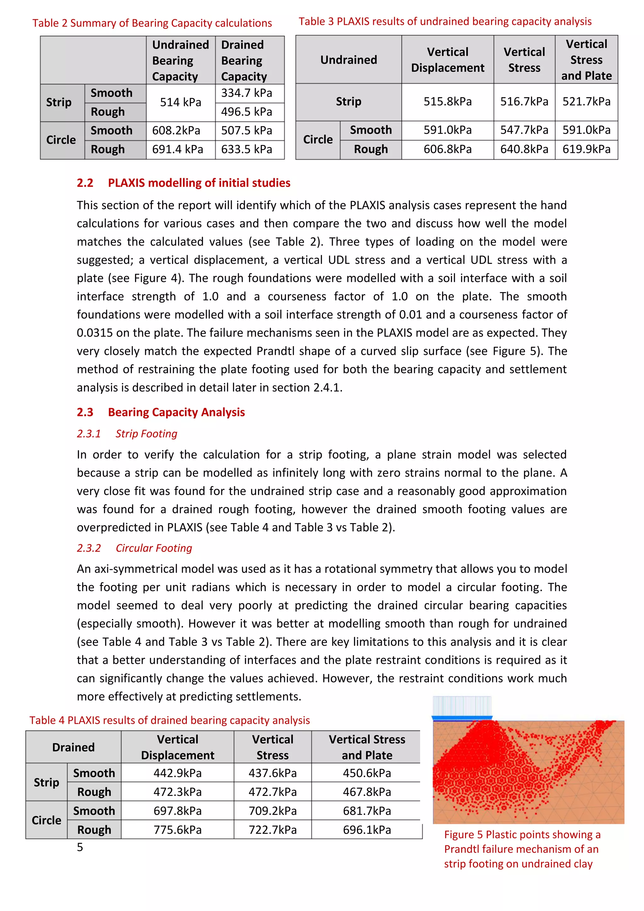
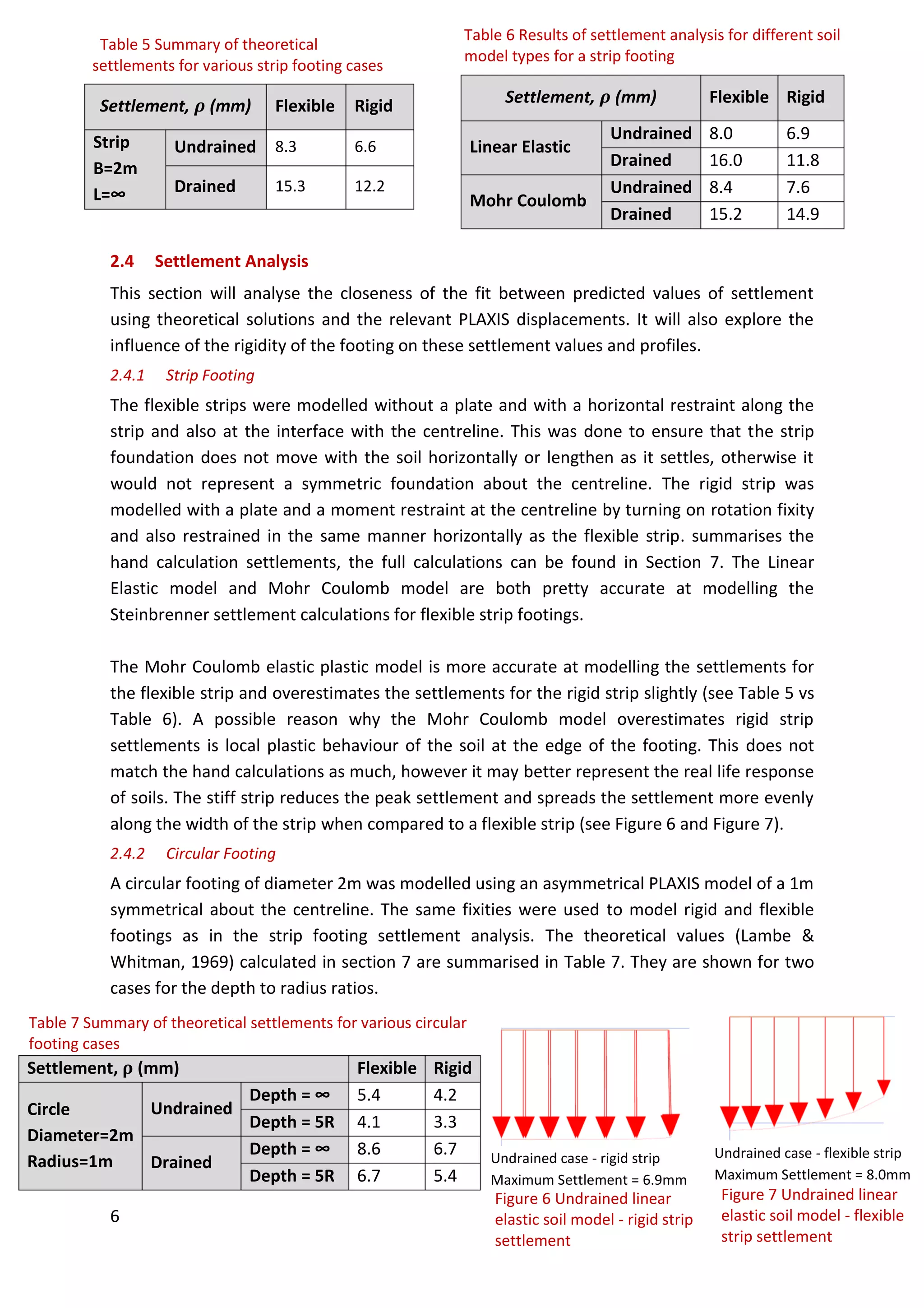
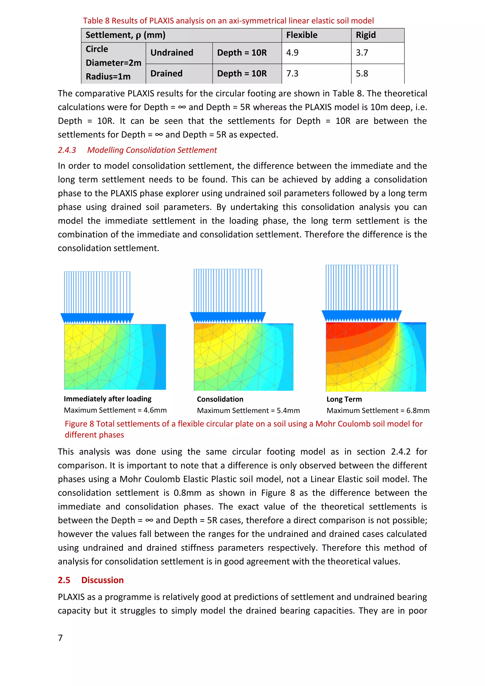
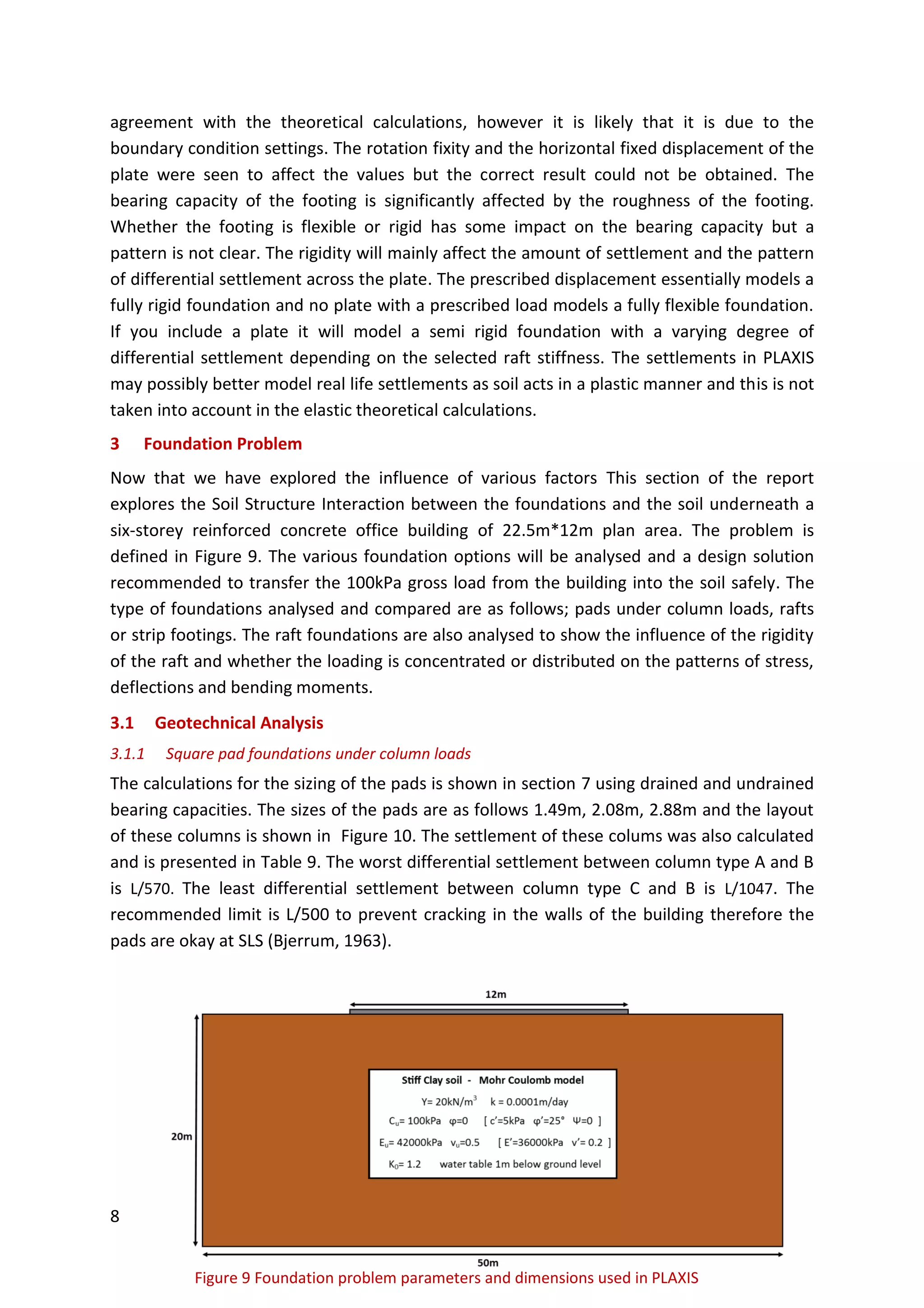
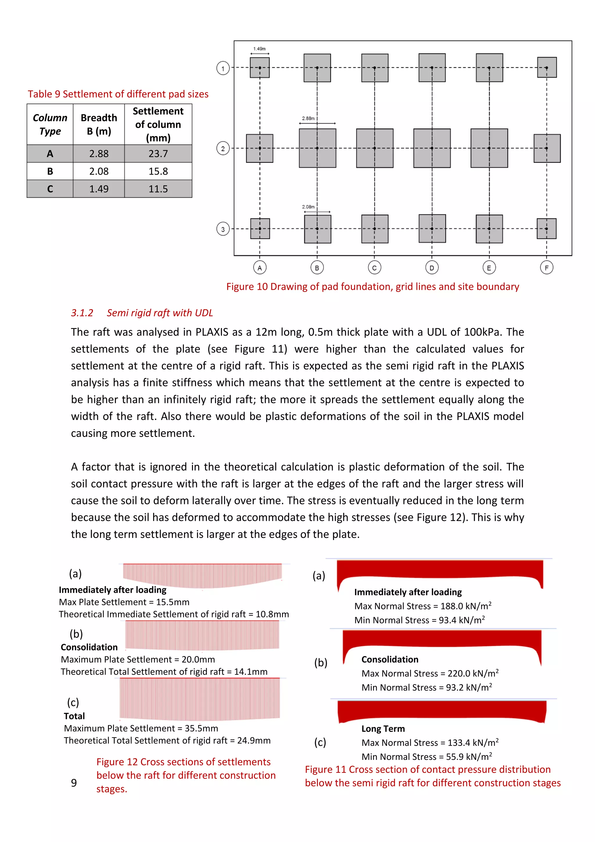
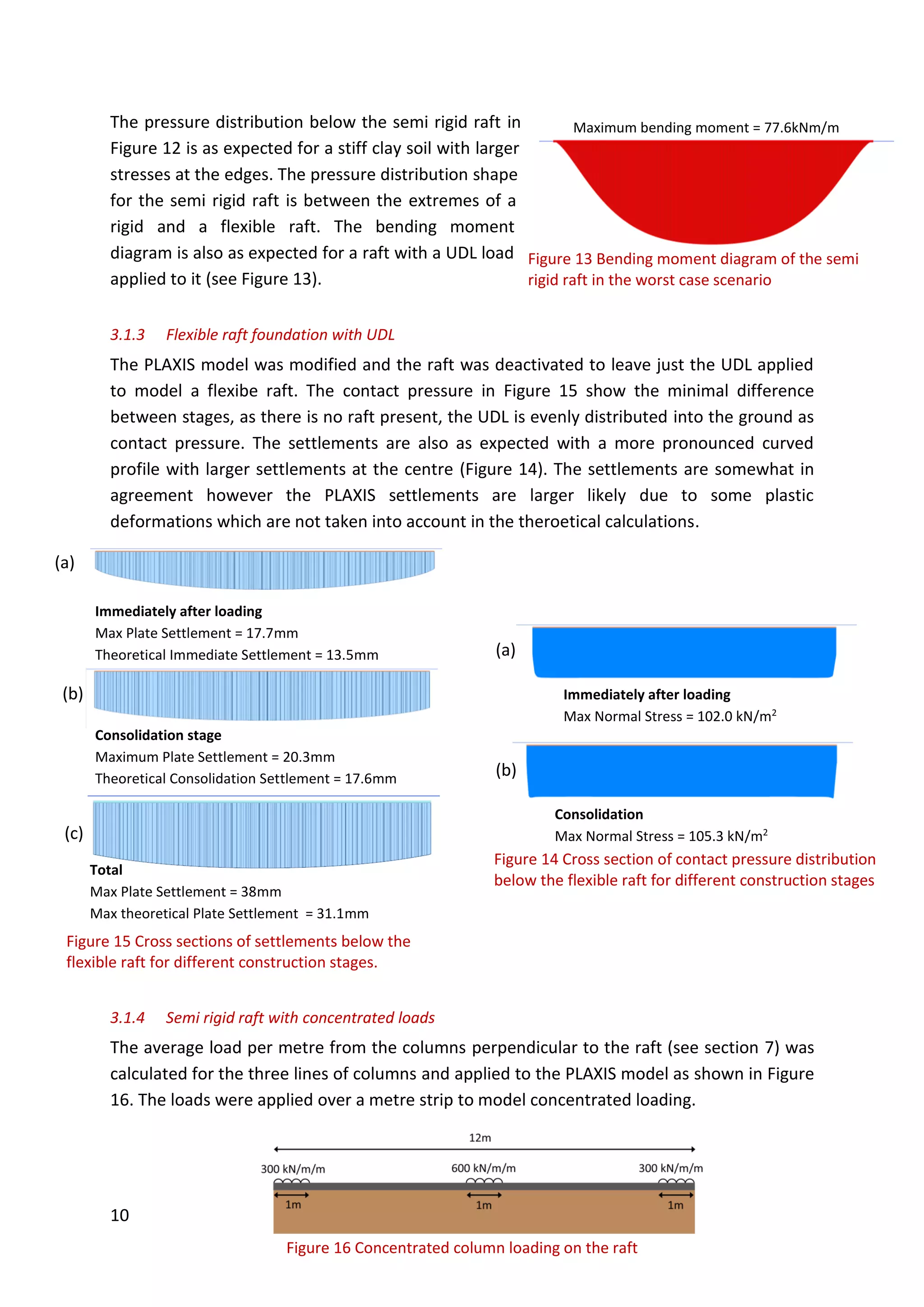
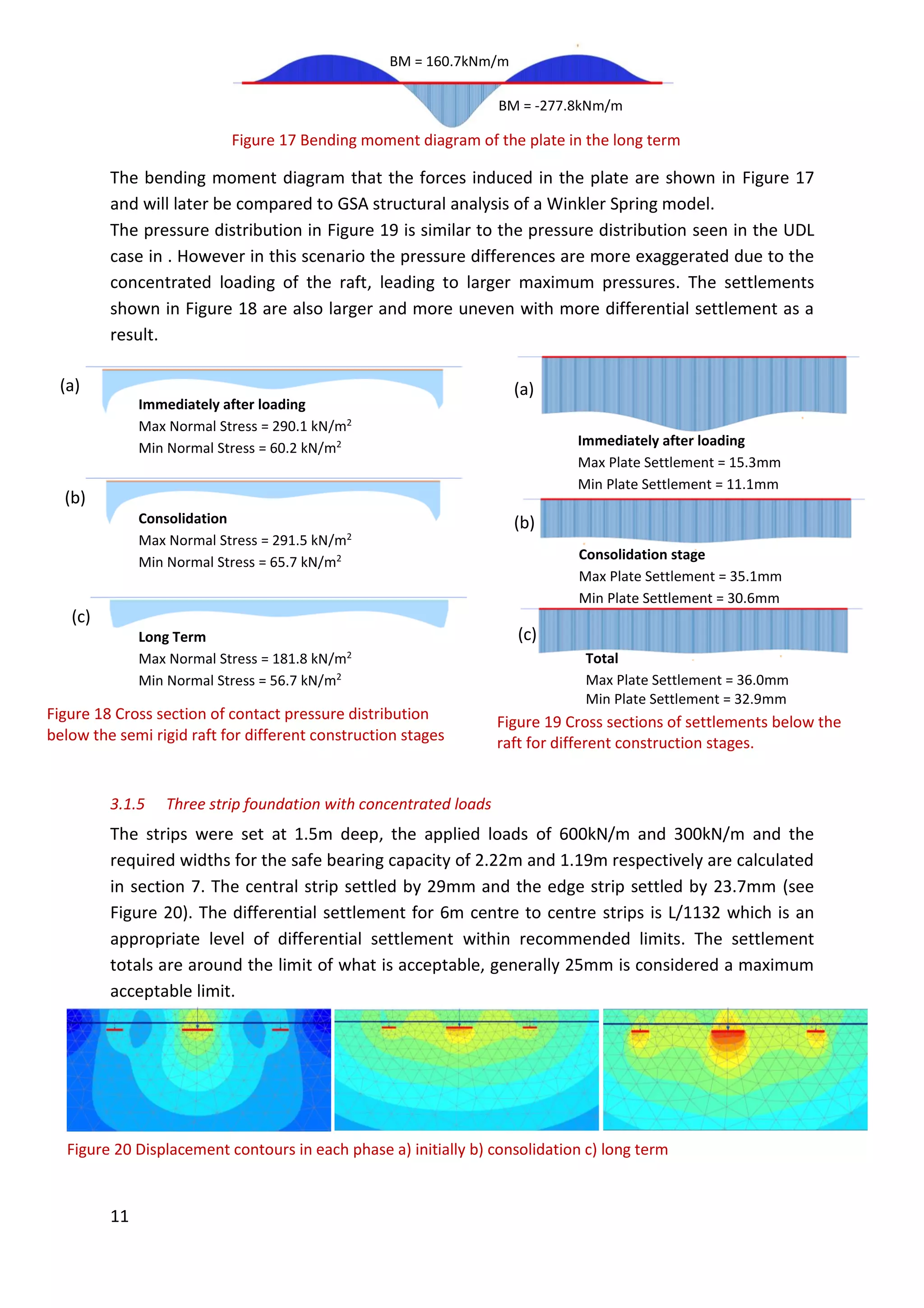
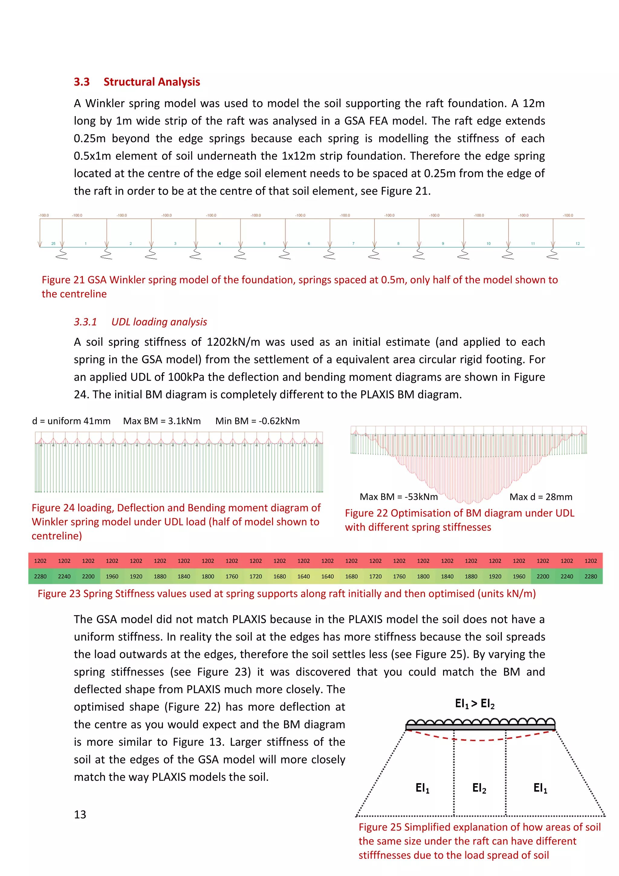
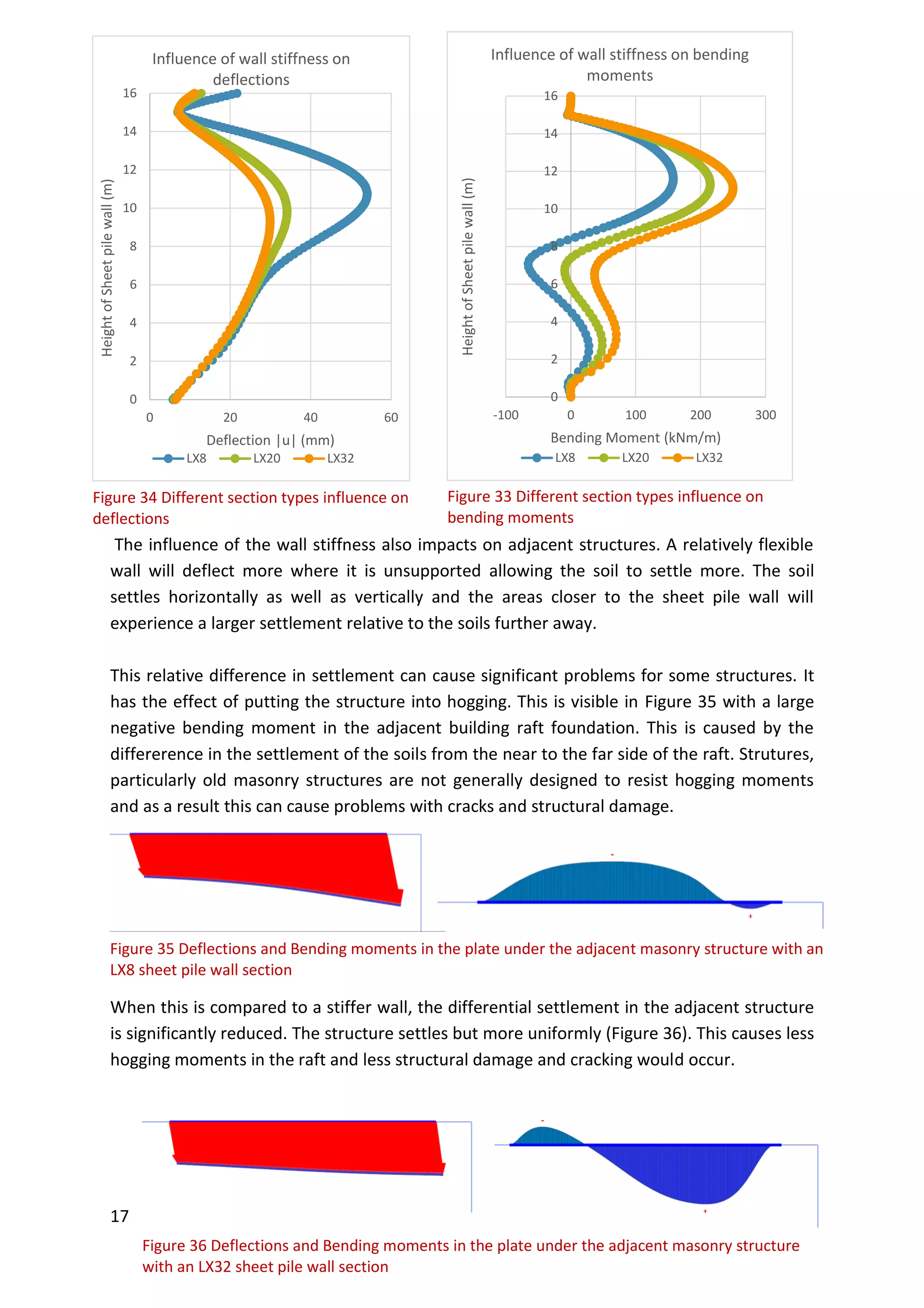
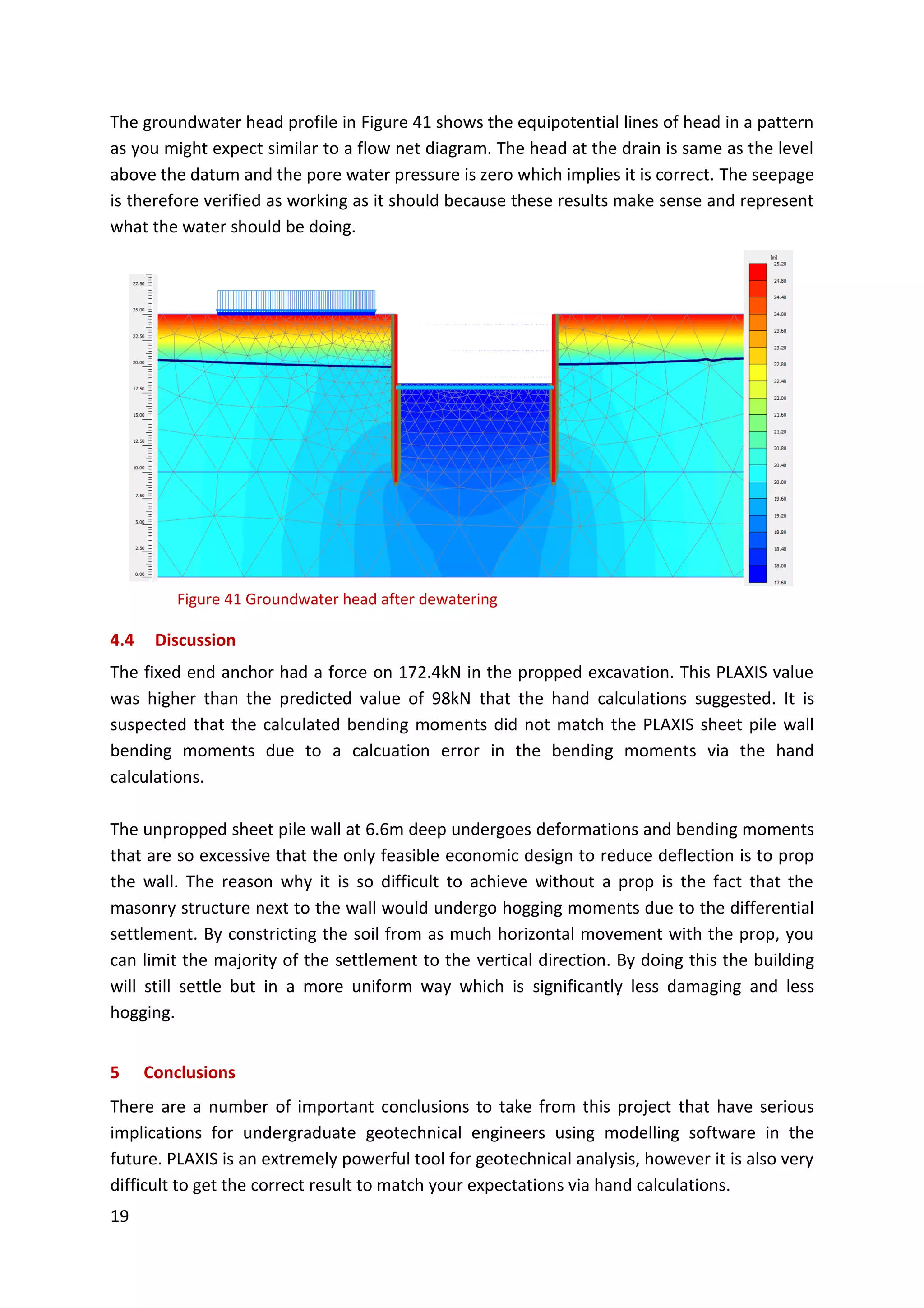
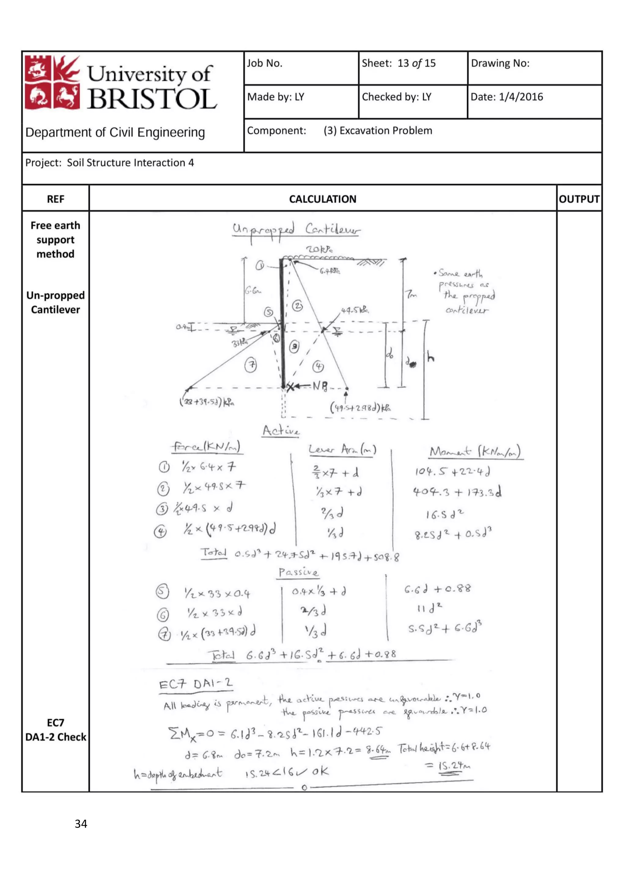
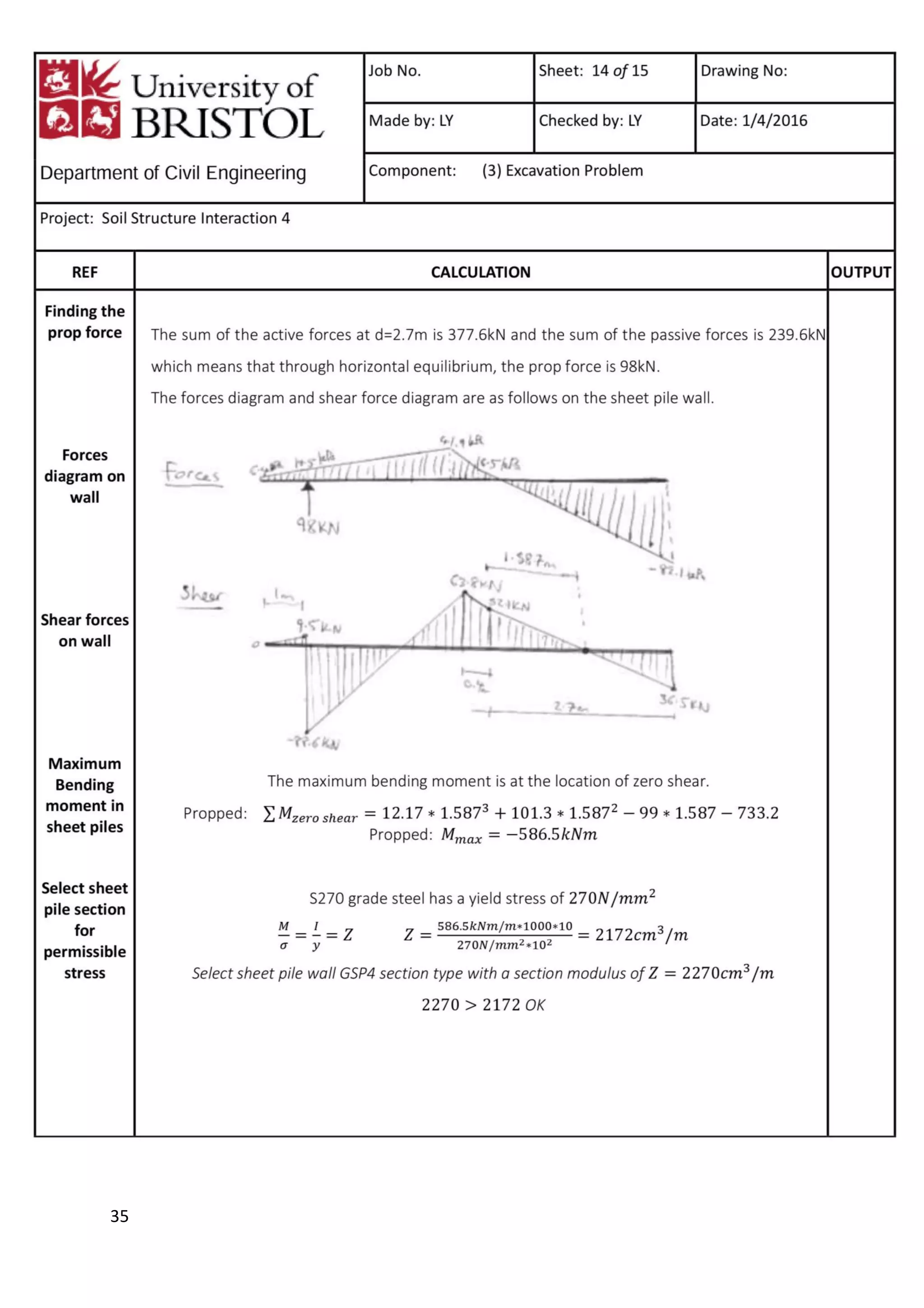
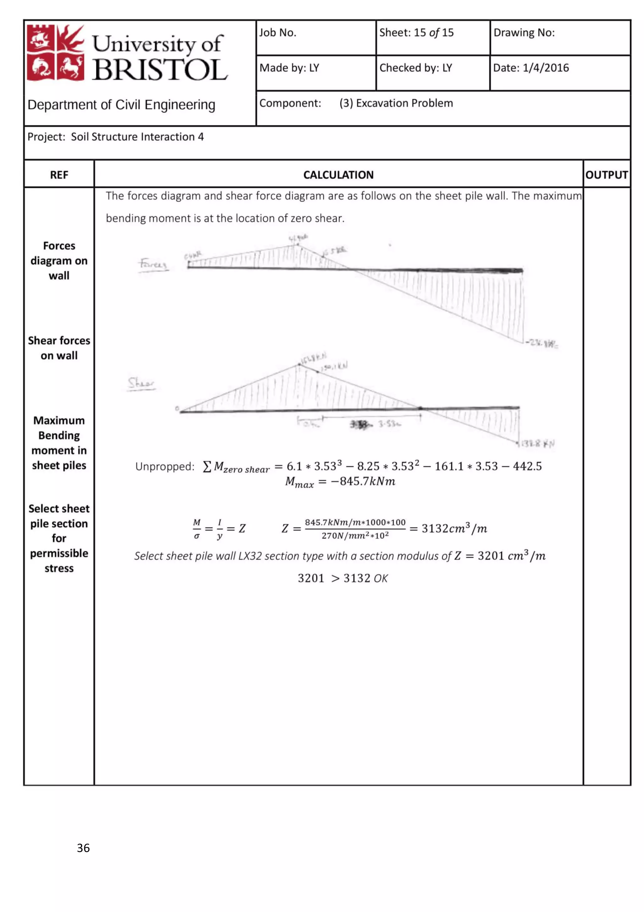
SlideShare a Scribd company logo
Department of Civil Engineering
Soil Structure Interaction 4
Leo Youngman
April 2016
2 Figure 1 Initial Studies parameters and dimensions used in PLAXIS
Table of Contents
1 Introduction...................................................................................................................2
2 Initial Studies .................................................................................................................2
3 Foundation Problem.......................................................................................................8
4 Excavation Problem......................................................................................................16
5 Conclusions..................................................................................................................19
6 References ...................................................................................................................21
7 Appendix – Calculations ...............................................................................................22
1 Introduction
This report is a study into finite element modelling of Soil Structure Interaction, the
applicability of these computer models to geotechnical problems and understanding the
limitations and benefits of using these models. The report is split into 3 sections exploring
the influence of various factors on finite element models and the difference this can make
when compared to hand calculations of the same problems. The hand calculations are
presented at the end of the report and referred to throughout the report and the key results
displayed and compared to the PLAXIS output.
2 Initial Studies
This section of the report compares the bearing capacity and settlement of foundations. By
comparing the PLAXIS analysis to hand calculations of known solutions, one can determine
the validity of using PLAXIS as a modelling tool for geotechnical problems. In addition to this,
the analysis is undertaken to determine the influence of the mesh, the boundary conditions
and distance from the boundaries to the foundation on the model. The analysis will also look
at the influence of the foundation stiffness and roughness and the depth of the water table.
The dimensions and parameters used in the PLAXIS model for the initial studies section are
shown in Figure 1. This is actually half of the 2m wide footing, however as it is symmetrical
we can split the problem into two to reduce the computation required.
3
2.1 Refining the Mesh
The mesh refinement in Table 1 shows that increasing the fineness of the global mesh
without local refinement is a very inefficient way of optimising the mesh. The change in the
% difference of the total force in the y axis (i.e. the bearing capacity of the footing) from very
coarse to fine is almost negligible. The influence of the general coarseness of the mesh alone
is insignificant.
Significant improvements in the accuracy of the mesh can be obtained with local
refinements at the footing location and at the left hand wall of the model (see Figure 3). This
is the area of highest stress and deformation, more refinement here increases the number
of elements thereby improving the accuracy of the mesh at the most important areas of
large stress gradients.
The selected mesh type for further analysis is a medium refined global mesh with 6 local
refinements at the area of interest. This was preferred because the mesh was accurate
enough with a 1.2% difference between the expected value and the PLAXIS output. Figure 2
describes how further refinement of the mesh does not provide significant increases in
accuracy, however they use a significant number of extra elements.
Description
of Mesh
Number of
refinements
No. of
Elements
PLAXIS Bearing
Capacity - Fy (kN)
Calculated
Bearing Capacity
(kN)
Percentage
Difference
Very Coarse 0 74 557.3 514 8.08%
Medium 0 212 556.7 514 7.98%
Fine 0 433 556.6 514 7.96%
Very Coarse 4 177 547.1 514 6.24%
Coarse 4 508 534.9 514 3.99%
Medium 4 519 533.4 514 3.70%
Very Coarse 6 514 529.6 514 2.99%
Coarse 6 1082 525.3 514 2.17%
Medium 6 1473 520.2 514 1.20%
Very Coarse 8 665 527.6 514 2.61%
Coarse 8 1279 525.1 514 2.14%
Medium 8 1882 523.3 514 1.79%
Medium Maximum 4956 522.1 514 1.56%
Table 1 Process of refinement of the mesh
Cartesian Total Stresses 𝝈 𝒚𝒚 (kN/m2)
Figure 3 Example of PLAXIS output with a coarse
mesh and some refinement at the left edge
Figure 2 Diminishing returns on accuracy with mesh fineness
R² = 0.7759
0%
1%
2%
3%
4%
5%
6%
7%
8%
9%
10%
0 1000 2000 3000 4000 5000
PercentageDifferencein
BearingCapacities
Number of Elements
Mesh Refinement Optimisation
4
Figure 4 Three loading cases: Applied displacement, flexible plate and semi-rigid plate
This mesh optimisation enables PLAXIS to calculate the output in the most efficient manner
whilst getting a reasonably accurate result. This can become a significant when undertaking
analysis of more complicated geotechnical models. The calculation time can become
significantly long that optimisation is required to save time and reduce the quantity of data
created. For each new model a mesh refinement should be completed and analysed for
accuracy against hand calculations.
2.1.1 Influence of Distance to Boundaries
When a model is run with model boundaries close to the area of influence of the foundation
the boundary will interact with the stresses in soil and alter the solution. Therefore it is
important to vary the distance to the boundaries and determine an appropriate distance
from the footing. In Figure 3 the cartesian stress contours are shown and it can be seen that
by moving the right hand boundary closer, it could have an impact on the stress distribution.
If the boundary was located anywhere closer than the 2m width of the footing, the wall
would interact with the stress bulb underneath the footing. Generally in geotechnical
modelling it is reccomended to leave at least 1-2 times the width of the footing spacing to
the boundaries. It can be non conservative otherwise as the boundaries provide a more rigid
support than other soils. Beyond 1-2 times the width, the differences are minimal as strains
are approaching zero (although they never reach zero).
2.1.2 Influence of Boundary Fixities
The model in all of these calculations has the following default boundary fixities. Free at
surface, horizontal restraints on the vertical boundaries and horizontal and vertical restraints
at the horizontal boundary at the base. The boundary fixity was varied in order to determine
the influence of this factor on the output.
If the base boundary is not fixed the soil body has no support and the entire structure will
not be restrained vertically. This is essentially a requirement of soil modelling similar to the
way structural finite element models require nodal restraints to ensure that globally the
structure is restained so that it cannot act as a mechanism.
The left and right hand boundaries are only fixed horizontally to keep the soil body from
collapsing, if it has no boundary then it would not be modelling the restraint provided by all
the soil around it to infinity. In real soil, far away from a footing there would be negligable
horizontal movement which approximates to a fixed boundary. The soil should however be
free to move vertically because soil can consolidate, deflect and settle vertically in real life
under structures.
5
2.2 PLAXIS modelling of initial studies
This section of the report will identify which of the PLAXIS analysis cases represent the hand
calculations for various cases and then compare the two and discuss how well the model
matches the calculated values (see Table 2). Three types of loading on the model were
suggested; a vertical displacement, a vertical UDL stress and a vertical UDL stress with a
plate (see Figure 4). The rough foundations were modelled with a soil interface with a soil
interface strength of 1.0 and a courseness factor of 1.0 on the plate. The smooth
foundations were modelled with a soil interface strength of 0.01 and a courseness factor of
0.0315 on the plate. The failure mechanisms seen in the PLAXIS model are as expected. They
very closely match the expected Prandtl shape of a curved slip surface (see Figure 5). The
method of restraining the plate footing used for both the bearing capacity and settlement
analysis is described in detail later in section 2.4.1.
2.3 Bearing Capacity Analysis
2.3.1 Strip Footing
In order to verify the calculation for a strip footing, a plane strain model was selected
because a strip can be modelled as infinitely long with zero strains normal to the plane. A
very close fit was found for the undrained strip case and a reasonably good approximation
was found for a drained rough footing, however the drained smooth footing values are
overpredicted in PLAXIS (see Table 4 and Table 3 vs Table 2).
2.3.2 Circular Footing
An axi-symmetrical model was used as it has a rotational symmetry that allows you to model
the footing per unit radians which is necessary in order to model a circular footing. The
model seemed to deal very poorly at predicting the drained circular bearing capacities
(especially smooth). However it was better at modelling smooth than rough for undrained
(see Table 4 and Table 3 vs Table 2). There are key limitations to this analysis and it is clear
that a better understanding of interfaces and the plate restraint conditions is required as it
can significantly change the values achieved. However, the restraint conditions work much
more effectively at predicting settlements.
Table 2 Summary of Bearing Capacity calculations
Undrained
Bearing
Capacity
Drained
Bearing
Capacity
Strip
Smooth
514 kPa
334.7 kPa
Rough 496.5 kPa
Circle
Smooth 608.2kPa 507.5 kPa
Rough 691.4 kPa 633.5 kPa
Undrained
Vertical
Displacement
Vertical
Stress
Vertical
Stress
and Plate
Strip 515.8kPa 516.7kPa 521.7kPa
Circle
Smooth 591.0kPa 547.7kPa 591.0kPa
Rough 606.8kPa 640.8kPa 619.9kPa
Table 3 PLAXIS results of undrained bearing capacity analysis
Drained
Vertical
Displacement
Vertical
Stress
Vertical Stress
and Plate
Strip
Smooth 442.9kPa 437.6kPa 450.6kPa
Rough 472.3kPa 472.7kPa 467.8kPa
Circle
Smooth 697.8kPa 709.2kPa 681.7kPa
Rough 775.6kPa 722.7kPa 696.1kPa
Table 4 PLAXIS results of drained bearing capacity analysis
Figure 5 Plastic points showing a
Prandtl failure mechanism of an
strip footing on undrained clay
6
Settlement, 𝝆 (mm) Flexible Rigid
Strip
B=2m
L=∞
Undrained 8.3 6.6
Drained 15.3 12.2
Table 5 Summary of theoretical
settlements for various strip footing cases
2.4 Settlement Analysis
This section will analyse the closeness of the fit between predicted values of settlement
using theoretical solutions and the relevant PLAXIS displacements. It will also explore the
influence of the rigidity of the footing on these settlement values and profiles.
2.4.1 Strip Footing
The flexible strips were modelled without a plate and with a horizontal restraint along the
strip and also at the interface with the centreline. This was done to ensure that the strip
foundation does not move with the soil horizontally or lengthen as it settles, otherwise it
would not represent a symmetric foundation about the centreline. The rigid strip was
modelled with a plate and a moment restraint at the centreline by turning on rotation fixity
and also restrained in the same manner horizontally as the flexible strip. summarises the
hand calculation settlements, the full calculations can be found in Section 7. The Linear
Elastic model and Mohr Coulomb model are both pretty accurate at modelling the
Steinbrenner settlement calculations for flexible strip footings.
The Mohr Coulomb elastic plastic model is more accurate at modelling the settlements for
the flexible strip and overestimates the settlements for the rigid strip slightly (see Table 5 vs
Table 6). A possible reason why the Mohr Coulomb model overestimates rigid strip
settlements is local plastic behaviour of the soil at the edge of the footing. This does not
match the hand calculations as much, however it may better represent the real life response
of soils. The stiff strip reduces the peak settlement and spreads the settlement more evenly
along the width of the strip when compared to a flexible strip (see Figure 6 and Figure 7).
2.4.2 Circular Footing
A circular footing of diameter 2m was modelled using an asymmetrical PLAXIS model of a 1m
symmetrical about the centreline. The same fixities were used to model rigid and flexible
footings as in the strip footing settlement analysis. The theoretical values (Lambe &
Whitman, 1969) calculated in section 7 are summarised in Table 7. They are shown for two
cases for the depth to radius ratios.
Table 6 Results of settlement analysis for different soil
model types for a strip footing
Settlement, 𝝆 (mm) Flexible Rigid
Linear Elastic
Undrained 8.0 6.9
Drained 16.0 11.8
Mohr Coulomb
Undrained 8.4 7.6
Drained 15.2 14.9
Undrained case - rigid strip
Maximum Settlement = 6.9mm
Figure 6 Undrained linear
elastic soil model - rigid strip
settlement
Settlement, 𝛒 (mm) Flexible Rigid
Circle
Diameter=2m
Radius=1m
Undrained
Depth = ∞ 5.4 4.2
Depth = 5R 4.1 3.3
Drained
Depth = ∞ 8.6 6.7
Depth = 5R 6.7 5.4
Table 7 Summary of theoretical settlements for various circular
footing cases
Undrained case - flexible strip
Maximum Settlement = 8.0mm
Figure 7 Undrained linear
elastic soil model - flexible
strip settlement
7
The comparative PLAXIS results for the circular footing are shown in Table 8. The theoretical
calculations were for Depth = ∞ and Depth = 5R whereas the PLAXIS model is 10m deep, i.e.
Depth = 10R. It can be seen that the settlements for Depth = 10R are between the
settlements for Depth = ∞ and Depth = 5R as expected.
2.4.3 Modelling Consolidation Settlement
In order to model consolidation settlement, the difference between the immediate and the
long term settlement needs to be found. This can be achieved by adding a consolidation
phase to the PLAXIS phase explorer using undrained soil parameters followed by a long term
phase using drained soil parameters. By undertaking this consolidation analysis you can
model the immediate settlement in the loading phase, the long term settlement is the
combination of the immediate and consolidation settlement. Therefore the difference is the
consolidation settlement.
This analysis was done using the same circular footing model as in section 2.4.2 for
comparison. It is important to note that a difference is only observed between the different
phases using a Mohr Coulomb Elastic Plastic soil model, not a Linear Elastic soil model. The
consolidation settlement is 0.8mm as shown in Figure 8 as the difference between the
immediate and consolidation phases. The exact value of the theoretical settlements is
between the Depth = ∞ and Depth = 5R cases, therefore a direct comparison is not possible;
however the values fall between the ranges for the undrained and drained cases calculated
using undrained and drained stiffness parameters respectively. Therefore this method of
analysis for consolidation settlement is in good agreement with the theoretical values.
2.5 Discussion
PLAXIS as a programme is relatively good at predictions of settlement and undrained bearing
capacity but it struggles to simply model the drained bearing capacities. They are in poor
Settlement, 𝛒 (mm) Flexible Rigid
Circle
Diameter=2m
Radius=1m
Undrained Depth = 10R 4.9 3.7
Drained Depth = 10R 7.3 5.8
Table 8 Results of PLAXIS analysis on an axi-symmetrical linear elastic soil model
Figure 8 Total settlements of a flexible circular plate on a soil using a Mohr Coulomb soil model for
different phases
Immediately after loading
Maximum Settlement = 4.6mm
Consolidation
Maximum Settlement = 5.4mm
Long Term
Maximum Settlement = 6.8mm
8
Figure 9 Foundation problem parameters and dimensions used in PLAXIS
agreement with the theoretical calculations, however it is likely that it is due to the
boundary condition settings. The rotation fixity and the horizontal fixed displacement of the
plate were seen to affect the values but the correct result could not be obtained. The
bearing capacity of the footing is significantly affected by the roughness of the footing.
Whether the footing is flexible or rigid has some impact on the bearing capacity but a
pattern is not clear. The rigidity will mainly affect the amount of settlement and the pattern
of differential settlement across the plate. The prescribed displacement essentially models a
fully rigid foundation and no plate with a prescribed load models a fully flexible foundation.
If you include a plate it will model a semi rigid foundation with a varying degree of
differential settlement depending on the selected raft stiffness. The settlements in PLAXIS
may possibly better model real life settlements as soil acts in a plastic manner and this is not
taken into account in the elastic theoretical calculations.
3 Foundation Problem
Now that we have explored the influence of various factors This section of the report
explores the Soil Structure Interaction between the foundations and the soil underneath a
six-storey reinforced concrete office building of 22.5m*12m plan area. The problem is
defined in Figure 9. The various foundation options will be analysed and a design solution
recommended to transfer the 100kPa gross load from the building into the soil safely. The
type of foundations analysed and compared are as follows; pads under column loads, rafts
or strip footings. The raft foundations are also analysed to show the influence of the rigidity
of the raft and whether the loading is concentrated or distributed on the patterns of stress,
deflections and bending moments.
3.1 Geotechnical Analysis
3.1.1 Square pad foundations under column loads
The calculations for the sizing of the pads is shown in section 7 using drained and undrained
bearing capacities. The sizes of the pads are as follows 1.49m, 2.08m, 2.88m and the layout
of these columns is shown in Figure 10. The settlement of these colums was also calculated
and is presented in Table 9. The worst differential settlement between column type A and B
is L/570. The least differential settlement between column type C and B is L/1047. The
recommended limit is L/500 to prevent cracking in the walls of the building therefore the
pads are okay at SLS (Bjerrum, 1963).
9
Column
Type
Breadth
B (m)
Settlement
of column
(mm)
A 2.88 23.7
B 2.08 15.8
C 1.49 11.5
Table 9 Settlement of different pad sizes
3.1.2 Semi rigid raft with UDL
The raft was analysed in PLAXIS as a 12m long, 0.5m thick plate with a UDL of 100kPa. The
settlements of the plate (see Figure 11) were higher than the calculated values for
settlement at the centre of a rigid raft. This is expected as the semi rigid raft in the PLAXIS
analysis has a finite stiffness which means that the settlement at the centre is expected to
be higher than an infinitely rigid raft; the more it spreads the settlement equally along the
width of the raft. Also there would be plastic deformations of the soil in the PLAXIS model
causing more settlement.
A factor that is ignored in the theoretical calculation is plastic deformation of the soil. The
soil contact pressure with the raft is larger at the edges of the raft and the larger stress will
cause the soil to deform laterally over time. The stress is eventually reduced in the long term
because the soil has deformed to accommodate the high stresses (see Figure 12). This is why
the long term settlement is larger at the edges of the plate.
Figure 11 Cross section of contact pressure distribution
below the semi rigid raft for different construction stages
(a)
(b)
Long Term
Max Normal Stress = 133.4 kN/m2
Min Normal Stress = 55.9 kN/m2
Consolidation
Max Normal Stress = 220.0 kN/m2
Min Normal Stress = 93.2 kN/m2
Immediately after loading
Max Normal Stress = 188.0 kN/m2
Min Normal Stress = 93.4 kN/m2
(c)
Immediately after loading
Max Plate Settlement = 15.5mm
Theoretical Immediate Settlement of rigid raft = 10.8mm
Consolidation
Maximum Plate Settlement = 20.0mm
Theoretical Total Settlement of rigid raft = 14.1mm
(a)
(b)
Figure 12 Cross sections of settlements
below the raft for different construction
stages.
(c)
Total
Maximum Plate Settlement = 35.5mm
Theoretical Total Settlement of rigid raft = 24.9mm
Figure 10 Drawing of pad foundation, grid lines and site boundary
10
Figure 16 Concentrated column loading on the raft
The pressure distribution below the semi rigid raft in
Figure 12 is as expected for a stiff clay soil with larger
stresses at the edges. The pressure distribution shape
for the semi rigid raft is between the extremes of a
rigid and a flexible raft. The bending moment
diagram is also as expected for a raft with a UDL load
applied to it (see Figure 13).
3.1.3 Flexible raft foundation with UDL
The PLAXIS model was modified and the raft was deactivated to leave just the UDL applied
to model a flexibe raft. The contact pressure in Figure 15 show the minimal difference
between stages, as there is no raft present, the UDL is evenly distributed into the ground as
contact pressure. The settlements are also as expected with a more pronounced curved
profile with larger settlements at the centre (Figure 14). The settlements are somewhat in
agreement however the PLAXIS settlements are larger likely due to some plastic
deformations which are not taken into account in the theroetical calculations.
3.1.4 Semi rigid raft with concentrated loads
The average load per metre from the columns perpendicular to the raft (see section 7) was
calculated for the three lines of columns and applied to the PLAXIS model as shown in Figure
16. The loads were applied over a metre strip to model concentrated loading.
Figure 14 Cross section of contact pressure distribution
below the flexible raft for different construction stages
(a)
(b)
Consolidation
Max Normal Stress = 105.3 kN/m2
Immediately after loading
Max Normal Stress = 102.0 kN/m2
Total
Max Plate Settlement = 38mm
Max theoretical Plate Settlement = 31.1mm
Consolidation stage
Maximum Plate Settlement = 20.3mm
Theoretical Consolidation Settlement = 17.6mm
Immediately after loading
Max Plate Settlement = 17.7mm
Theoretical Immediate Settlement = 13.5mm
(a)
(b)
(c)
Figure 15 Cross sections of settlements below the
flexible raft for different construction stages.
Maximum bending moment = 77.6kNm/m
Figure 13 Bending moment diagram of the semi
rigid raft in the worst case scenario
11
Figure 17 Bending moment diagram of the plate in the long term
BM = -277.8kNm/m
BM = 160.7kNm/m
The bending moment diagram that the forces induced in the plate are shown in Figure 17
and will later be compared to GSA structural analysis of a Winkler Spring model.
The pressure distribution in Figure 19 is similar to the pressure distribution seen in the UDL
case in . However in this scenario the pressure differences are more exaggerated due to the
concentrated loading of the raft, leading to larger maximum pressures. The settlements
shown in Figure 18 are also larger and more uneven with more differential settlement as a
result.
3.1.5 Three strip foundation with concentrated loads
The strips were set at 1.5m deep, the applied loads of 600kN/m and 300kN/m and the
required widths for the safe bearing capacity of 2.22m and 1.19m respectively are calculated
in section 7. The central strip settled by 29mm and the edge strip settled by 23.7mm (see
Figure 20). The differential settlement for 6m centre to centre strips is L/1132 which is an
appropriate level of differential settlement within recommended limits. The settlement
totals are around the limit of what is acceptable, generally 25mm is considered a maximum
acceptable limit.
(a)
(b)
Long Term
Max Normal Stress = 181.8 kN/m2
Min Normal Stress = 56.7 kN/m2
Consolidation
Max Normal Stress = 291.5 kN/m2
Min Normal Stress = 65.7 kN/m2
Immediately after loading
Max Normal Stress = 290.1 kN/m2
Min Normal Stress = 60.2 kN/m2
(c)
Figure 18 Cross section of contact pressure distribution
below the semi rigid raft for different construction stages
Figure 20 Displacement contours in each phase a) initially b) consolidation c) long term
Total
Max Plate Settlement = 36.0mm
Min Plate Settlement = 32.9mm
Consolidation stage
Max Plate Settlement = 35.1mm
Min Plate Settlement = 30.6mm
Immediately after loading
Max Plate Settlement = 15.3mm
Min Plate Settlement = 11.1mm
(a)
(b)
(c)
Figure 19 Cross sections of settlements below the
raft for different construction stages.
12
3.2 Selection of foundation type
3.2.1 Quick estimation of material volumes
The pads and strips were assumed to be 0.5m thick:
 The pad foundations are 4*(0.5m*(2.88m)2) + 10*((0.5m*(2.08m)2) +
4*((0.5m*(1.49m)2) = 42.7m3 of concrete
 The strip foundations are 2*(0.5m*1.2m*22.5m) + 1*(0.5m*2m*22.5m) = 49.5m3 of
concrete
 The raft foundation is 0.5m*12m*22.5m = 135m3 of concrete
3.2.2 Settlement comparisons
1. The settlements of the semi rigid raft with a UDL is 35.5mm. However with the
concentrated loads on the semi rigid raft, the settlements are 36mm. The raft with the
concentrated load case is more similar to the real life situation of column loading than
the UDL case. These settlements are high but probably just acceptable. The raft has a
differential settlement of 3mm which over a 3m distance between the highest and
lowest points equates to L/1000. This is well within acceptable differential settlement
limits.
2. The strip foundations settle 29mm and 23.7mm which is slightly beyond reccomended
limits but the size of the central strip could be increased to optimise this. The
differential settlements between the central and edge strips is L/1132.
3. The pad foundations were found to have settlements of 23.7mm, 15.8mm, 11.5mm
which are within the 25mm suggested limits. however the worst case differential
settlements were considerably worse (L/570) than for the other foundation types.
3.2.3 Justification of decision
The raft could be justified if there was a basement that required waterproofing however for
this application it is reccomended that strip foundations are used. They provide low values
of settlement, differential settlement and volumes of concrete required. The pads provide
lower settlement but significantly worse differential settlements close to the limit at which
cracking occurs. This is due to heavily loaded columns being located at short distances to the
least loaded columns.
The strip design could also be optimised with a larger central strip to reduce its settlement
to ensure it is within the recommeded 25mm limit. Another consideration is ease of
construction, the formwork required for the pad foundations is complex and more time
consuming and expensive to construct. However, at 1.5m deep it may require sloped
excavation or a propped excavation to reach the strip foundation level. This is because
working at this depth without propping is unsafe.
One possible disadvantage of the strip foundation reccomended is that it is at 1.5m deep
which is relatively deep and there would have to be a suspended ground slab anyway so the
savings in the foundation concrete may be negated by the extra structural concrete
compared to a raft that also acted as a ground floor slab.
13
Figure 25 Simplified explanation of how areas of soil
the same size under the raft can have different
stifffnesses due to the load spread of soil
3.3 Structural Analysis
A Winkler spring model was used to model the soil supporting the raft foundation. A 12m
long by 1m wide strip of the raft was analysed in a GSA FEA model. The raft edge extends
0.25m beyond the edge springs because each spring is modelling the stiffness of each
0.5x1m element of soil underneath the 1x12m strip foundation. Therefore the edge spring
located at the centre of the edge soil element needs to be spaced at 0.25m from the edge of
the raft in order to be at the centre of that soil element, see Figure 21.
3.3.1 UDL loading analysis
A soil spring stiffness of 1202kN/m was used as an initial estimate (and applied to each
spring in the GSA model) from the settlement of a equivalent area circular rigid footing. For
an applied UDL of 100kPa the deflection and bending moment diagrams are shown in Figure
24. The initial BM diagram is completely different to the PLAXIS BM diagram.
The GSA model did not match PLAXIS because in the PLAXIS model the soil does not have a
uniform stiffness. In reality the soil at the edges has more stiffness because the soil spreads
the load outwards at the edges, therefore the soil settles less (see Figure 25). By varying the
spring stiffnesses (see Figure 23) it was discovered that you could match the BM and
deflected shape from PLAXIS much more closely. The
optimised shape (Figure 22) has more deflection at
the centre as you would expect and the BM diagram
is more similar to Figure 13. Larger stiffness of the
soil at the edges of the GSA model will more closely
match the way PLAXIS models the soil.
Figure 21 GSA Winkler spring model of the foundation, springs spaced at 0.5m, only half of the model shown to
the centreline
d = uniform 41mm
Figure 24 loading, Deflection and Bending moment diagram of
Winkler spring model under UDL load (half of model shown to
centreline)
Max BM = 3.1kNm Min BM = -0.62kNm
1202 1202 1202 1202 1202 1202 1202 1202 1202 1202 1202 1202 1202 1202 1202 1202 1202 1202 1202 1202 1202 1202 1202 1202
2280 2240 2200 1960 1920 1880 1840 1800 1760 1720 1680 1640 1640 1680 1720 1760 1800 1840 1880 1920 1960 2200 2240 2280
Figure 23 Spring Stiffness values used at spring supports along raft initially and then optimised (units kN/m)
Figure 22 Optimisation of BM diagram under UDL
with different spring stiffnesses
Max BM = -53kNm Max d = 28mm
14
3.3.2 Concentrated Loading analysis
The same concentrated loads from the PLAXIS were applied to the GSA model as shown in
Figure 26. The deflections and bending moments are similar in shape but the values are
quite different. The optimised spring stiffnesses were used to change the BM profile to
match the PLAXIS result more closely. The BM and deflections in Figure 28 are much closer
to those from PLAXIS shown in Figure 17 and Figure 18.
The spring stiffness was optimised to be larger at the locations of the concentrated loads
(Figure 27). This more closely matches the PLAXIS result because of the load spread of the
soils directly under the loads. As with the UDL case, the load spread increases the soil
stiffness locally as it is supported by the soil around it and therefore there is a less
pronounced deflected shape underneath the concentrated loads compared to Figure 26.
By varying the soil stiffness, you can more accurately model differential settlements if you
were to apply these to a structural FE model of a building. The purpose of this structural
analysis is to introduce the concept of differential settlement modelling and how it could be
applied to structural models of buildings to check members for the stresses this may induce.
1202 1202 1202 1202 1202 1202 1202 1202 1202 1202 1202 1202 1202 1202 1202 1202 1202 1202 1202 1202 1202 1202 1202 1202
2325 2325 1725 1125 600 600 600 600 975 1575 2325 2325 2325 2325 1575 975 600 600 600 600 1125 1725 2325 2325
Figure 27 Spring Stiffness values used at spring supports along the raft initially and then optimised (units kN/m)
Figure 28 Optimisation of BM diagram under concentrated loads with different spring stiffnesses
Minimum BM = -171kNm
Maximum BM = 137kNm
Min d = 35mm
Max d = 39mm
Figure 26 Loading, deflection and bending moment diagram
of Winkler spring model under concentrated loading
Minimum BM = -155kNm
Maximum BM = 255kNm
Min d = 38.5mm
Max d = 51.0mm
15 Figure 30 Excavation problem parameters and dimensions used in PLAXIS
3.3.3 Influence of raft stiffness
By varying the stiffness of the raft under the concentrated loading we can see the variation
in the moment distribution as a result (Figure 29). This is the influence of the relative
stiffness of the raft to the soil. A stiffer raft has larger moments but deflects less. There
seems to be a point at which increasing the stiffness of the raft no longer has much of an
impact on the moment distribution, this is suspected to be because the raft is already very
rigid at 2m thick and as a result the deflected shape and the moments do not vary very much
with an increase in thickness. The dimensionless flexibility in the calculation for a 0.5m raft
was 3.04 implying a relatively flexible raft however the increase in raft thickness beyond
0.5m does not change the moment distribution that much. This implies that 0.5m is at the
limit of diminishing returns on thickness increase. It is unlikely to significantly reduce
differential settlement at a raft thickness larger than 0.5m.
-200
-150
-100
-50
0
50
100
150
200
0 2 4 6 8 10 12
Moment(kNm)
Length along raft (m)
Influence of stiffness of the raft on the moment distribution
Raft 0.1m deep
Raft 0.2m deep
Raft 0.5m deep
Raft 1m deep
Raft 2m deep
Figure 29 Influence of the raft thickness on the moment distribution under concentrated loading
16
4 Excavation Problem
This section of the report will explore the Soil Structure
Interaction between an existing masonry structure and
a nearby excavation. The influence of the sheet pile
section and a propping structure was investigated. The
foundation dimensions and parameters used in PLAXIS
are shown in Figure 30. A propped and an unpropped
sheet pile wall will be investigated and compared to
theoretical calculations.
4.1 Propped excavation
The propped excavation was modelled in PLAXIS with fixed end anchors and excavated to
6m plus an overdig of 0.6m in stages. The water table was lowered globally to 7m deep.
4.1.1 Comparison of horizontal stresses
The horizontal stresses in the theoretical calculations of earth pressures are an indealisation
of the actual earth pressures. In reality they are not completely triangular distributions
becasuse the stiffness of the wall varies the amount of deflection which causes interaction
with the soil and a different stress profile along the length. The active earth pressures are in
relatively good agreement along the length of the wall apart from at the location of the fixed
prop which increases local stresses (see Figure 31). The passive earth pressures however are
in poor agreement. This is possibly as a result of the difference in the PLAXIS model from the
theoretical situation. The model has 2 sheet pile walls which are both spreading the active
earth pressure loads horizontally into the soil on the passive side. This is shown in Figure 32.
This interaction beween the load spread shows why the passive stress profiles do not
accurately match the theoretical calculations.
4.1.2 Influence of stiffness of the wall
An increase in wall stiffness reduces the wall deflections where the wall is unsupported by
the soil. The deflection patterns are similar where the passive soil is located (Figure 34). The
stiffness of the wall also has an effect on the bending moments in the wall. A stiffer wall
attracts larger positive bending moments to the areas of large deflections because it is
resisting the deflections and high shear at that location (Figure 33).
Figure 32 Effective horizontal stresses σ’xx
Figure 31 Horizontal stress comparison on either
side of the sheet pile wall
0
2
4
6
8
10
12
14
16
-200 -100 0 100
Heightofsheetpilewall(m)
Effective Normal Stress, σ'N (kPa)
Earth pressures for propped
cantilever from PLAXIS
PLAXIS active earth pressure
PLAXIS passive earth pressures
Theoretical active eath pressures
Theoretical passive earth pressures
17
Figure 36 Deflections and Bending moments in the plate under the adjacent masonry structure
with an LX32 sheet pile wall section
The influence of the wall stiffness also impacts on adjacent structures. A relatively flexible
wall will deflect more where it is unsupported allowing the soil to settle more. The soil
settles horizontally as well as vertically and the areas closer to the sheet pile wall will
experience a larger settlement relative to the soils further away.
This relative difference in settlement can cause significant problems for some structures. It
has the effect of putting the structure into hogging. This is visible in Figure 35 with a large
negative bending moment in the adjacent building raft foundation. This is caused by the
differerence in the settlement of the soils from the near to the far side of the raft. Strutures,
particularly old masonry structures are not generally designed to resist hogging moments
and as a result this can cause problems with cracks and structural damage.
When this is compared to a stiffer wall, the differential settlement in the adjacent structure
is significantly reduced. The structure settles but more uniformly (Figure 36). This causes less
hogging moments in the raft and less structural damage and cracking would occur.
Figure 35 Deflections and Bending moments in the plate under the adjacent masonry structure with an
LX8 sheet pile wall section
0
2
4
6
8
10
12
14
16
0 20 40 60
HeightofSheetpilewall(m)
Deflection |u| (mm)
Influence of wall stiffness on
deflections
LX8 LX20 LX32
Figure 34 Different section types influence on
deflections
0
2
4
6
8
10
12
14
16
-100 0 100 200 300
HeightofSheetpilewall(m)
Bending Moment (kNm/m)
Influence of wall stiffness on bending
moments
LX8 LX20 LX32
Figure 33 Different section types influence on
bending moments
18
4.2 Unpropped excavation
The unpropped excavation was modelled in PLAXIS with 16m long sheet pile walls exactly
the same as the previous propped excavation. The water table in the PLAXIS analysis was at
the same level, the loading was the same and the wall was slightly deeper than the
theoretical calculation requirement of a 15.2m deep wall. However, the model still failed as
the soil body collapsed. The failure mechanism is shown in Figure 38 and the deformation of
the wall is shown in Figure 37. The wall is deflecting too much as a result of the large shear
forces and bending moments of the unpropped wall from the active earth pressures. The
analysis was also run with a very stiff sheet pile wall to 3m deeper and it the soil body still
failed. Clearly the depth of the excavation is too deep to not prop the wall. It is not
economically viable to keep increasing the embedment and the stifness of the wall, a much
cheaper and simpler solution is to prop the wall.
4.3 Seepage Analysis
4.3.1 Influence of dewatering inside the excavation
A repeat PLAXIS analysis was undertaken with a drain inside the excavation to lower the
water level only inside the excavation. This worked for the propped cantilever. The results of
this analysis can be used to verify whether PLAXIS is modelling seepage as it should. The
porewater pressures in Figure 40 have no discontiuity between the excavation and the main
soil body. There is a nice smooth change between the two areas, this means that the water
is modelled correctly. The groundwater flow in Figure 39 shows fast flow around the toe of
the shet pile which is as expected.
Figure 39 Groundwater flow after dewatering the
inside of the excavation
Figure 40 Pore water pressures after dewatering
excavation with a drain
Figure 37 Deformed mesh at failure
Figure 38 Plastic points showing failure mechanism of
unpropped excavation
19
The groundwater head profile in Figure 41 shows the equipotential lines of head in a pattern
as you might expect similar to a flow net diagram. The head at the drain is same as the level
above the datum and the pore water pressure is zero which implies it is correct. The seepage
is therefore verified as working as it should because these results make sense and represent
what the water should be doing.
4.4 Discussion
The fixed end anchor had a force on 172.4kN in the propped excavation. This PLAXIS value
was higher than the predicted value of 98kN that the hand calculations suggested. It is
suspected that the calculated bending moments did not match the PLAXIS sheet pile wall
bending moments due to a calcuation error in the bending moments via the hand
calculations.
The unpropped sheet pile wall at 6.6m deep undergoes deformations and bending moments
that are so excessive that the only feasible economic design to reduce deflection is to prop
the wall. The reason why it is so difficult to achieve without a prop is the fact that the
masonry structure next to the wall would undergo hogging moments due to the differential
settlement. By constricting the soil from as much horizontal movement with the prop, you
can limit the majority of the settlement to the vertical direction. By doing this the building
will still settle but in a more uniform way which is significantly less damaging and less
hogging.
5 Conclusions
There are a number of important conclusions to take from this project that have serious
implications for undergraduate geotechnical engineers using modelling software in the
future. PLAXIS is an extremely powerful tool for geotechnical analysis, however it is also very
difficult to get the correct result to match your expectations via hand calculations.
Figure 41 Groundwater head after dewatering
20
It is crucial that an engineer using these programs calculates the result that they are
expected to get using hand calculations and formulas. An undestanding of the expectations
of a whole variety of results is required. These include the bearing capacity, settlement,
deformed shape, bending moments, total and effective stresses, pore pressures, plastic
regions and failure mechanism. Experience of these is crucial to being able to know before
the program produces an output what it is likely to look like and how an incorrect model
could possibly look different to this. This is a crucial part of modelling through verififation.
It is also important to continually question all of selected PLAXIS settings you have decided
upon and check all of the inputs and outputs i.e. the model type and material parameters,
All of these results need to match your expectations from your accumulated engineering
knowledge, experience and research before you can be confident in the results.
As a software it has limitations and it is important to understand these. The bearing
capacities of various footings were quite challenging to match to the expected theoretical
values and as a result it is recommended in future to be extremely cautious about basing
design from these values. The settlements however are generally in good agreement and
PLAXIS would be a useful tool for modelling more complex structures with confidence that
the models are mostly in good agreement with the theoretical values.
When undertaking seepage analysis the groundwater flow boundary conditions are very
important to understand. Certain boundaries like the sheet pile walls and the base should
not allow seepage to occur. The output of the pore water pressures should also not have
discontinuities as this would not occur in the soil. It is very easy to quickly check the
groundwater head of the soil at different levels as a method verification of the
There are failure case studies where this methodology of verification and checks has not
been adhered to and caused loss of life as a result which emphasises how important it is to
get this right. These are often due to a lack of understanding of what the constitutive models
are doing, the This aside it is an extremely useful program for visualisation of expected
outputs, it is also very useful to be able to visually communicate these results to clients.
There are parts of the programme that are less understood and would require further
research to be confident in their use. The tension cutoff option for soils is unclear and is
notoriously difficult to model correctly, as shown in the Potts Rankine lecture. There are a
number of other modelling options that could be useful in the future such as the material
strength reduction analysis to failure, dynamic loading that could be used to model SSI
during seismic loading. Judging by the complexity of the simpler options, these other options
would only be reccomended with the guidance of a highly skilled and experienced user.
21
6 References
Bjerrum, L., 1963. Contribution to the discussion. ECSHFE, 2(6), pp. 135-137.
Bolton, M. & Lau, C., 1993. Vertical Bearing Capacity factors for circular and strip footings on
Mohr-Coulomb soil. Canadian Geotechnics Journal , Issue 30, pp. 1024-1033.
Bowles, J. E., 1987. Elastic foundation settlement on sand deposits. Journal of Geotechnical
Engineering, 113(8), pp. 846-860.
Caquot, A. I. & Kerisel, J., 1948. Tables for the calculation of passive pressure, active
pressure, and bearing capacity of foundations.. Libraire du Bureau des Longitudes, p. 120.
Chattopadhyay, B., 2014. Foundation Engineering. s.l.:PHI Learning Pvt. Ltd..
Ibraim, E., 2015. Geotechnics 3 Lecture Notes. Bristol: Department of Civil Engineering
University of Bristol.
Lambe, T. & Whitman, R., 1969. Soil Mechanics. New York: Wiley.
Müller-Breslau, H., 1906. Erddruck auf Stutzmauern. Stuttgart: Alfred Kroner.
Potts, D. M., 2003. Numerical analysis: a virtual dream or practical reality?. Geotechnique,
53(6), pp. 535-573.
Prandtl, L., 1921. Uber die Eindringungsfestigkeit plasticher Baustoffe und die Festigkeit von
Schneiden. Zeitschrift fur Angewandte Mathematik und Mechanik, 1(1), pp. 15-20.
S Gourvenec, M. R. O. K., 2006. Undrained Bearing Capacity of Square and Rectangular
Footings. INTERNATIONAL JOURNAL OF GEOMECHANICS ASCE, 6(3), pp. 147-157.
Salgado, R., 2007. The Engineering of Foundations. s.l.:McGraw Hill.
Steinbrenner, W., 1934. Tafeln zur setzungsberschnung. Die Strasse, Volume 1, pp. 121-124.
Terzaghi, K., 1943. Theoretical Soil Mechanics. New York: Wiley.
Waite, D. & Williams, B., 1993. The Design and Construction of Sheet Piled Cofferdams.
London: Construction Industry Research and Information Association CIRIA.
22
7 Appendix – Calculations
23
24
25
26
27
28
29
30
31
32
33
34
35
36

More Related Content

What's hot

SPT CORRELATIONS.ppt
SPT CORRELATIONS.pptSPT CORRELATIONS.ppt
SPT CORRELATIONS.ppt
satheeskumarv2
 
L6 - Beam Design.pdf
L6 - Beam Design.pdfL6 - Beam Design.pdf
L6 - Beam Design.pdf
IsmaeelWaseethAhmed
 
A study on characterization of compressive strength. seminar pptx
A study on characterization of compressive strength. seminar pptxA study on characterization of compressive strength. seminar pptx
A study on characterization of compressive strength. seminar pptx
naveen_envi
 
200832154 brosur-spun-pile-wika-2011
200832154 brosur-spun-pile-wika-2011200832154 brosur-spun-pile-wika-2011
200832154 brosur-spun-pile-wika-2011
algifakhri bagus maulana
 
Chapter 5 strip.pptx STRIP METHOD FOR SLAB
Chapter 5 strip.pptx STRIP METHOD FOR SLABChapter 5 strip.pptx STRIP METHOD FOR SLAB
Chapter 5 strip.pptx STRIP METHOD FOR SLAB
tekalign24
 
Base Isolation(2000.12.28)
Base Isolation(2000.12.28)Base Isolation(2000.12.28)
Base Isolation(2000.12.28)
mahadianto
 
Chapter 19
Chapter 19Chapter 19
Chapter 19
SantistebanCampos
 
W.h.mosley, j.h.bungey. reinforced concrete design book
W.h.mosley, j.h.bungey. reinforced concrete design bookW.h.mosley, j.h.bungey. reinforced concrete design book
W.h.mosley, j.h.bungey. reinforced concrete design book
Reyam AL Mousawi
 
One way slab design by Sabuj Chowdhury, Lecturer, Department of CIvil Enginee...
One way slab design by Sabuj Chowdhury, Lecturer, Department of CIvil Enginee...One way slab design by Sabuj Chowdhury, Lecturer, Department of CIvil Enginee...
One way slab design by Sabuj Chowdhury, Lecturer, Department of CIvil Enginee...
Md Rizwanul Islam Riaj
 
Kbb_UII_Arsi 14_ a kiki cs_kayu_okky
Kbb_UII_Arsi 14_ a kiki cs_kayu_okkyKbb_UII_Arsi 14_ a kiki cs_kayu_okky
Kbb_UII_Arsi 14_ a kiki cs_kayu_okky
Kiki Zakiyah
 
Bab i
Bab iBab i
Pile Eccentricity Analysis for 2 Columns Combined Pilecap
Pile Eccentricity Analysis for 2 Columns Combined PilecapPile Eccentricity Analysis for 2 Columns Combined Pilecap
Pile Eccentricity Analysis for 2 Columns Combined Pilecap
azhar ahmad
 
Lecture 8 raft foundation
Lecture 8 raft foundationLecture 8 raft foundation
Lecture 8 raft foundation
Dr.Abdulmannan Orabi
 
Concrete Mix Design Manual
Concrete Mix Design ManualConcrete Mix Design Manual
Concrete Mix Design Manual
Nirman Pokharel
 
EFFECT OF DIFFERENT MOLARITY OF ALKALINE ACTIVATOR ON FLY ASH BASED CONCRETE
EFFECT OF DIFFERENT MOLARITY OF ALKALINE ACTIVATOR ON FLY ASH BASED CONCRETEEFFECT OF DIFFERENT MOLARITY OF ALKALINE ACTIVATOR ON FLY ASH BASED CONCRETE
EFFECT OF DIFFERENT MOLARITY OF ALKALINE ACTIVATOR ON FLY ASH BASED CONCRETE
UMESHCHAKRABORTY1
 
Cube test REPORT - DCC2042
Cube test REPORT - DCC2042Cube test REPORT - DCC2042
Cube test REPORT - DCC2042
Pavitrah Segaran
 
Marshall Mix Design: Lab Report
Marshall Mix Design: Lab ReportMarshall Mix Design: Lab Report
Marshall Mix Design: Lab Report
Priyansh Singh
 
Seismic analysis of vertical irregular multistoried building
Seismic analysis of vertical irregular multistoried buildingSeismic analysis of vertical irregular multistoried building
Seismic analysis of vertical irregular multistoried building
eSAT Journals
 
Retaining Wall_Lecture.ppt
Retaining Wall_Lecture.pptRetaining Wall_Lecture.ppt
Retaining Wall_Lecture.ppt
atul625446
 
ultimate bearing capacity of shallow foundations: special cases
ultimate bearing capacity of shallow foundations: special casesultimate bearing capacity of shallow foundations: special cases
ultimate bearing capacity of shallow foundations: special cases
Mehmet Akin
 

What's hot (20)

SPT CORRELATIONS.ppt
SPT CORRELATIONS.pptSPT CORRELATIONS.ppt
SPT CORRELATIONS.ppt
 
L6 - Beam Design.pdf
L6 - Beam Design.pdfL6 - Beam Design.pdf
L6 - Beam Design.pdf
 
A study on characterization of compressive strength. seminar pptx
A study on characterization of compressive strength. seminar pptxA study on characterization of compressive strength. seminar pptx
A study on characterization of compressive strength. seminar pptx
 
200832154 brosur-spun-pile-wika-2011
200832154 brosur-spun-pile-wika-2011200832154 brosur-spun-pile-wika-2011
200832154 brosur-spun-pile-wika-2011
 
Chapter 5 strip.pptx STRIP METHOD FOR SLAB
Chapter 5 strip.pptx STRIP METHOD FOR SLABChapter 5 strip.pptx STRIP METHOD FOR SLAB
Chapter 5 strip.pptx STRIP METHOD FOR SLAB
 
Base Isolation(2000.12.28)
Base Isolation(2000.12.28)Base Isolation(2000.12.28)
Base Isolation(2000.12.28)
 
Chapter 19
Chapter 19Chapter 19
Chapter 19
 
W.h.mosley, j.h.bungey. reinforced concrete design book
W.h.mosley, j.h.bungey. reinforced concrete design bookW.h.mosley, j.h.bungey. reinforced concrete design book
W.h.mosley, j.h.bungey. reinforced concrete design book
 
One way slab design by Sabuj Chowdhury, Lecturer, Department of CIvil Enginee...
One way slab design by Sabuj Chowdhury, Lecturer, Department of CIvil Enginee...One way slab design by Sabuj Chowdhury, Lecturer, Department of CIvil Enginee...
One way slab design by Sabuj Chowdhury, Lecturer, Department of CIvil Enginee...
 
Kbb_UII_Arsi 14_ a kiki cs_kayu_okky
Kbb_UII_Arsi 14_ a kiki cs_kayu_okkyKbb_UII_Arsi 14_ a kiki cs_kayu_okky
Kbb_UII_Arsi 14_ a kiki cs_kayu_okky
 
Bab i
Bab iBab i
Bab i
 
Pile Eccentricity Analysis for 2 Columns Combined Pilecap
Pile Eccentricity Analysis for 2 Columns Combined PilecapPile Eccentricity Analysis for 2 Columns Combined Pilecap
Pile Eccentricity Analysis for 2 Columns Combined Pilecap
 
Lecture 8 raft foundation
Lecture 8 raft foundationLecture 8 raft foundation
Lecture 8 raft foundation
 
Concrete Mix Design Manual
Concrete Mix Design ManualConcrete Mix Design Manual
Concrete Mix Design Manual
 
EFFECT OF DIFFERENT MOLARITY OF ALKALINE ACTIVATOR ON FLY ASH BASED CONCRETE
EFFECT OF DIFFERENT MOLARITY OF ALKALINE ACTIVATOR ON FLY ASH BASED CONCRETEEFFECT OF DIFFERENT MOLARITY OF ALKALINE ACTIVATOR ON FLY ASH BASED CONCRETE
EFFECT OF DIFFERENT MOLARITY OF ALKALINE ACTIVATOR ON FLY ASH BASED CONCRETE
 
Cube test REPORT - DCC2042
Cube test REPORT - DCC2042Cube test REPORT - DCC2042
Cube test REPORT - DCC2042
 
Marshall Mix Design: Lab Report
Marshall Mix Design: Lab ReportMarshall Mix Design: Lab Report
Marshall Mix Design: Lab Report
 
Seismic analysis of vertical irregular multistoried building
Seismic analysis of vertical irregular multistoried buildingSeismic analysis of vertical irregular multistoried building
Seismic analysis of vertical irregular multistoried building
 
Retaining Wall_Lecture.ppt
Retaining Wall_Lecture.pptRetaining Wall_Lecture.ppt
Retaining Wall_Lecture.ppt
 
ultimate bearing capacity of shallow foundations: special cases
ultimate bearing capacity of shallow foundations: special casesultimate bearing capacity of shallow foundations: special cases
ultimate bearing capacity of shallow foundations: special cases
 

Similar to Soil-Structure-Interaction-4-Coursework---Leo-Youngman-15-16

Young_Stress_Analyst_Competetion_Entry
Young_Stress_Analyst_Competetion_EntryYoung_Stress_Analyst_Competetion_Entry
Young_Stress_Analyst_Competetion_Entry
Luqmaan Fazal Ph.D.
 
Fixity depth of offshore piles in elastoplastic soft clay under dynamic load
Fixity depth of offshore piles in elastoplastic soft clay under dynamic loadFixity depth of offshore piles in elastoplastic soft clay under dynamic load
Fixity depth of offshore piles in elastoplastic soft clay under dynamic load
eSAT Journals
 
Fixity depth of offshore piles in elastoplastic soft clay under dynamic load
Fixity depth of offshore piles in elastoplastic soft clay under dynamic loadFixity depth of offshore piles in elastoplastic soft clay under dynamic load
Fixity depth of offshore piles in elastoplastic soft clay under dynamic load
eSAT Journals
 
Slip Line Field Method
Slip Line Field MethodSlip Line Field Method
Slip Line Field Method
Santosh Verma
 
A032010107
A032010107A032010107
A032010107
inventionjournals
 
Theoretical study for r.c. columns strengthened with gfrp with different main...
Theoretical study for r.c. columns strengthened with gfrp with different main...Theoretical study for r.c. columns strengthened with gfrp with different main...
Theoretical study for r.c. columns strengthened with gfrp with different main...
Ahmed Ebid
 
Unit 1 notes-final
Unit 1 notes-finalUnit 1 notes-final
Unit 1 notes-final
jagadish108
 
Linear And Nonlinear Analytical Modeling of Laminated Composite Beams In Thre...
Linear And Nonlinear Analytical Modeling of Laminated Composite Beams In Thre...Linear And Nonlinear Analytical Modeling of Laminated Composite Beams In Thre...
Linear And Nonlinear Analytical Modeling of Laminated Composite Beams In Thre...
researchinventy
 
FEDSM2013-16202
FEDSM2013-16202FEDSM2013-16202
FEDSM2013-16202
Praneetha Boppa
 
Atmospheric turbulent layer simulation for cfd unsteady inlet conditions
Atmospheric turbulent layer simulation for cfd unsteady inlet conditionsAtmospheric turbulent layer simulation for cfd unsteady inlet conditions
Atmospheric turbulent layer simulation for cfd unsteady inlet conditions
Stephane Meteodyn
 
H slabs
H slabsH slabs
H slabs
AbirMahmud34
 
ABAQUS simulation for consolidation of saturated soft soil in two-dimensional...
ABAQUS simulation for consolidation of saturated soft soil in two-dimensional...ABAQUS simulation for consolidation of saturated soft soil in two-dimensional...
ABAQUS simulation for consolidation of saturated soft soil in two-dimensional...
IJRES Journal
 
2016 optimisation a rear wing endplate in a rotating domain
2016 optimisation a rear wing endplate in a rotating domain2016 optimisation a rear wing endplate in a rotating domain
2016 optimisation a rear wing endplate in a rotating domain
Hashan Mendis
 
Analysis of stiffened isotropic and composite plate
Analysis of stiffened isotropic and composite plateAnalysis of stiffened isotropic and composite plate
Analysis of stiffened isotropic and composite plate
IRJET Journal
 
Texture and crack growth behaviour
Texture and crack growth behaviourTexture and crack growth behaviour
Texture and crack growth behaviour
Sum K
 
Texture and crack growth behaviour
Texture and crack growth behaviourTexture and crack growth behaviour
Texture and crack growth behaviour
Sum K
 
Texture and crack growth behaviour
Texture and crack growth behaviourTexture and crack growth behaviour
Texture and crack growth behaviour
Sum K
 
Eqe.2391 (1)
Eqe.2391 (1)Eqe.2391 (1)
Eqe.2391 (1)
andri priyanto
 
MSE490 FinalReport
MSE490 FinalReportMSE490 FinalReport
MSE490 FinalReport
Zhenjie Yao
 
Comparative Study on Anchorage in Reinforced Concrete Using Codes of Practice...
Comparative Study on Anchorage in Reinforced Concrete Using Codes of Practice...Comparative Study on Anchorage in Reinforced Concrete Using Codes of Practice...
Comparative Study on Anchorage in Reinforced Concrete Using Codes of Practice...
IJERA Editor
 

Similar to Soil-Structure-Interaction-4-Coursework---Leo-Youngman-15-16 (20)

Young_Stress_Analyst_Competetion_Entry
Young_Stress_Analyst_Competetion_EntryYoung_Stress_Analyst_Competetion_Entry
Young_Stress_Analyst_Competetion_Entry
 
Fixity depth of offshore piles in elastoplastic soft clay under dynamic load
Fixity depth of offshore piles in elastoplastic soft clay under dynamic loadFixity depth of offshore piles in elastoplastic soft clay under dynamic load
Fixity depth of offshore piles in elastoplastic soft clay under dynamic load
 
Fixity depth of offshore piles in elastoplastic soft clay under dynamic load
Fixity depth of offshore piles in elastoplastic soft clay under dynamic loadFixity depth of offshore piles in elastoplastic soft clay under dynamic load
Fixity depth of offshore piles in elastoplastic soft clay under dynamic load
 
Slip Line Field Method
Slip Line Field MethodSlip Line Field Method
Slip Line Field Method
 
A032010107
A032010107A032010107
A032010107
 
Theoretical study for r.c. columns strengthened with gfrp with different main...
Theoretical study for r.c. columns strengthened with gfrp with different main...Theoretical study for r.c. columns strengthened with gfrp with different main...
Theoretical study for r.c. columns strengthened with gfrp with different main...
 
Unit 1 notes-final
Unit 1 notes-finalUnit 1 notes-final
Unit 1 notes-final
 
Linear And Nonlinear Analytical Modeling of Laminated Composite Beams In Thre...
Linear And Nonlinear Analytical Modeling of Laminated Composite Beams In Thre...Linear And Nonlinear Analytical Modeling of Laminated Composite Beams In Thre...
Linear And Nonlinear Analytical Modeling of Laminated Composite Beams In Thre...
 
FEDSM2013-16202
FEDSM2013-16202FEDSM2013-16202
FEDSM2013-16202
 
Atmospheric turbulent layer simulation for cfd unsteady inlet conditions
Atmospheric turbulent layer simulation for cfd unsteady inlet conditionsAtmospheric turbulent layer simulation for cfd unsteady inlet conditions
Atmospheric turbulent layer simulation for cfd unsteady inlet conditions
 
H slabs
H slabsH slabs
H slabs
 
ABAQUS simulation for consolidation of saturated soft soil in two-dimensional...
ABAQUS simulation for consolidation of saturated soft soil in two-dimensional...ABAQUS simulation for consolidation of saturated soft soil in two-dimensional...
ABAQUS simulation for consolidation of saturated soft soil in two-dimensional...
 
2016 optimisation a rear wing endplate in a rotating domain
2016 optimisation a rear wing endplate in a rotating domain2016 optimisation a rear wing endplate in a rotating domain
2016 optimisation a rear wing endplate in a rotating domain
 
Analysis of stiffened isotropic and composite plate
Analysis of stiffened isotropic and composite plateAnalysis of stiffened isotropic and composite plate
Analysis of stiffened isotropic and composite plate
 
Texture and crack growth behaviour
Texture and crack growth behaviourTexture and crack growth behaviour
Texture and crack growth behaviour
 
Texture and crack growth behaviour
Texture and crack growth behaviourTexture and crack growth behaviour
Texture and crack growth behaviour
 
Texture and crack growth behaviour
Texture and crack growth behaviourTexture and crack growth behaviour
Texture and crack growth behaviour
 
Eqe.2391 (1)
Eqe.2391 (1)Eqe.2391 (1)
Eqe.2391 (1)
 
MSE490 FinalReport
MSE490 FinalReportMSE490 FinalReport
MSE490 FinalReport
 
Comparative Study on Anchorage in Reinforced Concrete Using Codes of Practice...
Comparative Study on Anchorage in Reinforced Concrete Using Codes of Practice...Comparative Study on Anchorage in Reinforced Concrete Using Codes of Practice...
Comparative Study on Anchorage in Reinforced Concrete Using Codes of Practice...
 

Soil-Structure-Interaction-4-Coursework---Leo-Youngman-15-16

  • 1. Department of Civil Engineering Soil Structure Interaction 4 Leo Youngman April 2016
  • 2. 2 Figure 1 Initial Studies parameters and dimensions used in PLAXIS Table of Contents 1 Introduction...................................................................................................................2 2 Initial Studies .................................................................................................................2 3 Foundation Problem.......................................................................................................8 4 Excavation Problem......................................................................................................16 5 Conclusions..................................................................................................................19 6 References ...................................................................................................................21 7 Appendix – Calculations ...............................................................................................22 1 Introduction This report is a study into finite element modelling of Soil Structure Interaction, the applicability of these computer models to geotechnical problems and understanding the limitations and benefits of using these models. The report is split into 3 sections exploring the influence of various factors on finite element models and the difference this can make when compared to hand calculations of the same problems. The hand calculations are presented at the end of the report and referred to throughout the report and the key results displayed and compared to the PLAXIS output. 2 Initial Studies This section of the report compares the bearing capacity and settlement of foundations. By comparing the PLAXIS analysis to hand calculations of known solutions, one can determine the validity of using PLAXIS as a modelling tool for geotechnical problems. In addition to this, the analysis is undertaken to determine the influence of the mesh, the boundary conditions and distance from the boundaries to the foundation on the model. The analysis will also look at the influence of the foundation stiffness and roughness and the depth of the water table. The dimensions and parameters used in the PLAXIS model for the initial studies section are shown in Figure 1. This is actually half of the 2m wide footing, however as it is symmetrical we can split the problem into two to reduce the computation required.
  • 3. 3 2.1 Refining the Mesh The mesh refinement in Table 1 shows that increasing the fineness of the global mesh without local refinement is a very inefficient way of optimising the mesh. The change in the % difference of the total force in the y axis (i.e. the bearing capacity of the footing) from very coarse to fine is almost negligible. The influence of the general coarseness of the mesh alone is insignificant. Significant improvements in the accuracy of the mesh can be obtained with local refinements at the footing location and at the left hand wall of the model (see Figure 3). This is the area of highest stress and deformation, more refinement here increases the number of elements thereby improving the accuracy of the mesh at the most important areas of large stress gradients. The selected mesh type for further analysis is a medium refined global mesh with 6 local refinements at the area of interest. This was preferred because the mesh was accurate enough with a 1.2% difference between the expected value and the PLAXIS output. Figure 2 describes how further refinement of the mesh does not provide significant increases in accuracy, however they use a significant number of extra elements. Description of Mesh Number of refinements No. of Elements PLAXIS Bearing Capacity - Fy (kN) Calculated Bearing Capacity (kN) Percentage Difference Very Coarse 0 74 557.3 514 8.08% Medium 0 212 556.7 514 7.98% Fine 0 433 556.6 514 7.96% Very Coarse 4 177 547.1 514 6.24% Coarse 4 508 534.9 514 3.99% Medium 4 519 533.4 514 3.70% Very Coarse 6 514 529.6 514 2.99% Coarse 6 1082 525.3 514 2.17% Medium 6 1473 520.2 514 1.20% Very Coarse 8 665 527.6 514 2.61% Coarse 8 1279 525.1 514 2.14% Medium 8 1882 523.3 514 1.79% Medium Maximum 4956 522.1 514 1.56% Table 1 Process of refinement of the mesh Cartesian Total Stresses 𝝈 𝒚𝒚 (kN/m2) Figure 3 Example of PLAXIS output with a coarse mesh and some refinement at the left edge Figure 2 Diminishing returns on accuracy with mesh fineness R² = 0.7759 0% 1% 2% 3% 4% 5% 6% 7% 8% 9% 10% 0 1000 2000 3000 4000 5000 PercentageDifferencein BearingCapacities Number of Elements Mesh Refinement Optimisation
  • 4. 4 Figure 4 Three loading cases: Applied displacement, flexible plate and semi-rigid plate This mesh optimisation enables PLAXIS to calculate the output in the most efficient manner whilst getting a reasonably accurate result. This can become a significant when undertaking analysis of more complicated geotechnical models. The calculation time can become significantly long that optimisation is required to save time and reduce the quantity of data created. For each new model a mesh refinement should be completed and analysed for accuracy against hand calculations. 2.1.1 Influence of Distance to Boundaries When a model is run with model boundaries close to the area of influence of the foundation the boundary will interact with the stresses in soil and alter the solution. Therefore it is important to vary the distance to the boundaries and determine an appropriate distance from the footing. In Figure 3 the cartesian stress contours are shown and it can be seen that by moving the right hand boundary closer, it could have an impact on the stress distribution. If the boundary was located anywhere closer than the 2m width of the footing, the wall would interact with the stress bulb underneath the footing. Generally in geotechnical modelling it is reccomended to leave at least 1-2 times the width of the footing spacing to the boundaries. It can be non conservative otherwise as the boundaries provide a more rigid support than other soils. Beyond 1-2 times the width, the differences are minimal as strains are approaching zero (although they never reach zero). 2.1.2 Influence of Boundary Fixities The model in all of these calculations has the following default boundary fixities. Free at surface, horizontal restraints on the vertical boundaries and horizontal and vertical restraints at the horizontal boundary at the base. The boundary fixity was varied in order to determine the influence of this factor on the output. If the base boundary is not fixed the soil body has no support and the entire structure will not be restrained vertically. This is essentially a requirement of soil modelling similar to the way structural finite element models require nodal restraints to ensure that globally the structure is restained so that it cannot act as a mechanism. The left and right hand boundaries are only fixed horizontally to keep the soil body from collapsing, if it has no boundary then it would not be modelling the restraint provided by all the soil around it to infinity. In real soil, far away from a footing there would be negligable horizontal movement which approximates to a fixed boundary. The soil should however be free to move vertically because soil can consolidate, deflect and settle vertically in real life under structures.
  • 5. 5 2.2 PLAXIS modelling of initial studies This section of the report will identify which of the PLAXIS analysis cases represent the hand calculations for various cases and then compare the two and discuss how well the model matches the calculated values (see Table 2). Three types of loading on the model were suggested; a vertical displacement, a vertical UDL stress and a vertical UDL stress with a plate (see Figure 4). The rough foundations were modelled with a soil interface with a soil interface strength of 1.0 and a courseness factor of 1.0 on the plate. The smooth foundations were modelled with a soil interface strength of 0.01 and a courseness factor of 0.0315 on the plate. The failure mechanisms seen in the PLAXIS model are as expected. They very closely match the expected Prandtl shape of a curved slip surface (see Figure 5). The method of restraining the plate footing used for both the bearing capacity and settlement analysis is described in detail later in section 2.4.1. 2.3 Bearing Capacity Analysis 2.3.1 Strip Footing In order to verify the calculation for a strip footing, a plane strain model was selected because a strip can be modelled as infinitely long with zero strains normal to the plane. A very close fit was found for the undrained strip case and a reasonably good approximation was found for a drained rough footing, however the drained smooth footing values are overpredicted in PLAXIS (see Table 4 and Table 3 vs Table 2). 2.3.2 Circular Footing An axi-symmetrical model was used as it has a rotational symmetry that allows you to model the footing per unit radians which is necessary in order to model a circular footing. The model seemed to deal very poorly at predicting the drained circular bearing capacities (especially smooth). However it was better at modelling smooth than rough for undrained (see Table 4 and Table 3 vs Table 2). There are key limitations to this analysis and it is clear that a better understanding of interfaces and the plate restraint conditions is required as it can significantly change the values achieved. However, the restraint conditions work much more effectively at predicting settlements. Table 2 Summary of Bearing Capacity calculations Undrained Bearing Capacity Drained Bearing Capacity Strip Smooth 514 kPa 334.7 kPa Rough 496.5 kPa Circle Smooth 608.2kPa 507.5 kPa Rough 691.4 kPa 633.5 kPa Undrained Vertical Displacement Vertical Stress Vertical Stress and Plate Strip 515.8kPa 516.7kPa 521.7kPa Circle Smooth 591.0kPa 547.7kPa 591.0kPa Rough 606.8kPa 640.8kPa 619.9kPa Table 3 PLAXIS results of undrained bearing capacity analysis Drained Vertical Displacement Vertical Stress Vertical Stress and Plate Strip Smooth 442.9kPa 437.6kPa 450.6kPa Rough 472.3kPa 472.7kPa 467.8kPa Circle Smooth 697.8kPa 709.2kPa 681.7kPa Rough 775.6kPa 722.7kPa 696.1kPa Table 4 PLAXIS results of drained bearing capacity analysis Figure 5 Plastic points showing a Prandtl failure mechanism of an strip footing on undrained clay
  • 6. 6 Settlement, 𝝆 (mm) Flexible Rigid Strip B=2m L=∞ Undrained 8.3 6.6 Drained 15.3 12.2 Table 5 Summary of theoretical settlements for various strip footing cases 2.4 Settlement Analysis This section will analyse the closeness of the fit between predicted values of settlement using theoretical solutions and the relevant PLAXIS displacements. It will also explore the influence of the rigidity of the footing on these settlement values and profiles. 2.4.1 Strip Footing The flexible strips were modelled without a plate and with a horizontal restraint along the strip and also at the interface with the centreline. This was done to ensure that the strip foundation does not move with the soil horizontally or lengthen as it settles, otherwise it would not represent a symmetric foundation about the centreline. The rigid strip was modelled with a plate and a moment restraint at the centreline by turning on rotation fixity and also restrained in the same manner horizontally as the flexible strip. summarises the hand calculation settlements, the full calculations can be found in Section 7. The Linear Elastic model and Mohr Coulomb model are both pretty accurate at modelling the Steinbrenner settlement calculations for flexible strip footings. The Mohr Coulomb elastic plastic model is more accurate at modelling the settlements for the flexible strip and overestimates the settlements for the rigid strip slightly (see Table 5 vs Table 6). A possible reason why the Mohr Coulomb model overestimates rigid strip settlements is local plastic behaviour of the soil at the edge of the footing. This does not match the hand calculations as much, however it may better represent the real life response of soils. The stiff strip reduces the peak settlement and spreads the settlement more evenly along the width of the strip when compared to a flexible strip (see Figure 6 and Figure 7). 2.4.2 Circular Footing A circular footing of diameter 2m was modelled using an asymmetrical PLAXIS model of a 1m symmetrical about the centreline. The same fixities were used to model rigid and flexible footings as in the strip footing settlement analysis. The theoretical values (Lambe & Whitman, 1969) calculated in section 7 are summarised in Table 7. They are shown for two cases for the depth to radius ratios. Table 6 Results of settlement analysis for different soil model types for a strip footing Settlement, 𝝆 (mm) Flexible Rigid Linear Elastic Undrained 8.0 6.9 Drained 16.0 11.8 Mohr Coulomb Undrained 8.4 7.6 Drained 15.2 14.9 Undrained case - rigid strip Maximum Settlement = 6.9mm Figure 6 Undrained linear elastic soil model - rigid strip settlement Settlement, 𝛒 (mm) Flexible Rigid Circle Diameter=2m Radius=1m Undrained Depth = ∞ 5.4 4.2 Depth = 5R 4.1 3.3 Drained Depth = ∞ 8.6 6.7 Depth = 5R 6.7 5.4 Table 7 Summary of theoretical settlements for various circular footing cases Undrained case - flexible strip Maximum Settlement = 8.0mm Figure 7 Undrained linear elastic soil model - flexible strip settlement
  • 7. 7 The comparative PLAXIS results for the circular footing are shown in Table 8. The theoretical calculations were for Depth = ∞ and Depth = 5R whereas the PLAXIS model is 10m deep, i.e. Depth = 10R. It can be seen that the settlements for Depth = 10R are between the settlements for Depth = ∞ and Depth = 5R as expected. 2.4.3 Modelling Consolidation Settlement In order to model consolidation settlement, the difference between the immediate and the long term settlement needs to be found. This can be achieved by adding a consolidation phase to the PLAXIS phase explorer using undrained soil parameters followed by a long term phase using drained soil parameters. By undertaking this consolidation analysis you can model the immediate settlement in the loading phase, the long term settlement is the combination of the immediate and consolidation settlement. Therefore the difference is the consolidation settlement. This analysis was done using the same circular footing model as in section 2.4.2 for comparison. It is important to note that a difference is only observed between the different phases using a Mohr Coulomb Elastic Plastic soil model, not a Linear Elastic soil model. The consolidation settlement is 0.8mm as shown in Figure 8 as the difference between the immediate and consolidation phases. The exact value of the theoretical settlements is between the Depth = ∞ and Depth = 5R cases, therefore a direct comparison is not possible; however the values fall between the ranges for the undrained and drained cases calculated using undrained and drained stiffness parameters respectively. Therefore this method of analysis for consolidation settlement is in good agreement with the theoretical values. 2.5 Discussion PLAXIS as a programme is relatively good at predictions of settlement and undrained bearing capacity but it struggles to simply model the drained bearing capacities. They are in poor Settlement, 𝛒 (mm) Flexible Rigid Circle Diameter=2m Radius=1m Undrained Depth = 10R 4.9 3.7 Drained Depth = 10R 7.3 5.8 Table 8 Results of PLAXIS analysis on an axi-symmetrical linear elastic soil model Figure 8 Total settlements of a flexible circular plate on a soil using a Mohr Coulomb soil model for different phases Immediately after loading Maximum Settlement = 4.6mm Consolidation Maximum Settlement = 5.4mm Long Term Maximum Settlement = 6.8mm
  • 8. 8 Figure 9 Foundation problem parameters and dimensions used in PLAXIS agreement with the theoretical calculations, however it is likely that it is due to the boundary condition settings. The rotation fixity and the horizontal fixed displacement of the plate were seen to affect the values but the correct result could not be obtained. The bearing capacity of the footing is significantly affected by the roughness of the footing. Whether the footing is flexible or rigid has some impact on the bearing capacity but a pattern is not clear. The rigidity will mainly affect the amount of settlement and the pattern of differential settlement across the plate. The prescribed displacement essentially models a fully rigid foundation and no plate with a prescribed load models a fully flexible foundation. If you include a plate it will model a semi rigid foundation with a varying degree of differential settlement depending on the selected raft stiffness. The settlements in PLAXIS may possibly better model real life settlements as soil acts in a plastic manner and this is not taken into account in the elastic theoretical calculations. 3 Foundation Problem Now that we have explored the influence of various factors This section of the report explores the Soil Structure Interaction between the foundations and the soil underneath a six-storey reinforced concrete office building of 22.5m*12m plan area. The problem is defined in Figure 9. The various foundation options will be analysed and a design solution recommended to transfer the 100kPa gross load from the building into the soil safely. The type of foundations analysed and compared are as follows; pads under column loads, rafts or strip footings. The raft foundations are also analysed to show the influence of the rigidity of the raft and whether the loading is concentrated or distributed on the patterns of stress, deflections and bending moments. 3.1 Geotechnical Analysis 3.1.1 Square pad foundations under column loads The calculations for the sizing of the pads is shown in section 7 using drained and undrained bearing capacities. The sizes of the pads are as follows 1.49m, 2.08m, 2.88m and the layout of these columns is shown in Figure 10. The settlement of these colums was also calculated and is presented in Table 9. The worst differential settlement between column type A and B is L/570. The least differential settlement between column type C and B is L/1047. The recommended limit is L/500 to prevent cracking in the walls of the building therefore the pads are okay at SLS (Bjerrum, 1963).
  • 9. 9 Column Type Breadth B (m) Settlement of column (mm) A 2.88 23.7 B 2.08 15.8 C 1.49 11.5 Table 9 Settlement of different pad sizes 3.1.2 Semi rigid raft with UDL The raft was analysed in PLAXIS as a 12m long, 0.5m thick plate with a UDL of 100kPa. The settlements of the plate (see Figure 11) were higher than the calculated values for settlement at the centre of a rigid raft. This is expected as the semi rigid raft in the PLAXIS analysis has a finite stiffness which means that the settlement at the centre is expected to be higher than an infinitely rigid raft; the more it spreads the settlement equally along the width of the raft. Also there would be plastic deformations of the soil in the PLAXIS model causing more settlement. A factor that is ignored in the theoretical calculation is plastic deformation of the soil. The soil contact pressure with the raft is larger at the edges of the raft and the larger stress will cause the soil to deform laterally over time. The stress is eventually reduced in the long term because the soil has deformed to accommodate the high stresses (see Figure 12). This is why the long term settlement is larger at the edges of the plate. Figure 11 Cross section of contact pressure distribution below the semi rigid raft for different construction stages (a) (b) Long Term Max Normal Stress = 133.4 kN/m2 Min Normal Stress = 55.9 kN/m2 Consolidation Max Normal Stress = 220.0 kN/m2 Min Normal Stress = 93.2 kN/m2 Immediately after loading Max Normal Stress = 188.0 kN/m2 Min Normal Stress = 93.4 kN/m2 (c) Immediately after loading Max Plate Settlement = 15.5mm Theoretical Immediate Settlement of rigid raft = 10.8mm Consolidation Maximum Plate Settlement = 20.0mm Theoretical Total Settlement of rigid raft = 14.1mm (a) (b) Figure 12 Cross sections of settlements below the raft for different construction stages. (c) Total Maximum Plate Settlement = 35.5mm Theoretical Total Settlement of rigid raft = 24.9mm Figure 10 Drawing of pad foundation, grid lines and site boundary
  • 10. 10 Figure 16 Concentrated column loading on the raft The pressure distribution below the semi rigid raft in Figure 12 is as expected for a stiff clay soil with larger stresses at the edges. The pressure distribution shape for the semi rigid raft is between the extremes of a rigid and a flexible raft. The bending moment diagram is also as expected for a raft with a UDL load applied to it (see Figure 13). 3.1.3 Flexible raft foundation with UDL The PLAXIS model was modified and the raft was deactivated to leave just the UDL applied to model a flexibe raft. The contact pressure in Figure 15 show the minimal difference between stages, as there is no raft present, the UDL is evenly distributed into the ground as contact pressure. The settlements are also as expected with a more pronounced curved profile with larger settlements at the centre (Figure 14). The settlements are somewhat in agreement however the PLAXIS settlements are larger likely due to some plastic deformations which are not taken into account in the theroetical calculations. 3.1.4 Semi rigid raft with concentrated loads The average load per metre from the columns perpendicular to the raft (see section 7) was calculated for the three lines of columns and applied to the PLAXIS model as shown in Figure 16. The loads were applied over a metre strip to model concentrated loading. Figure 14 Cross section of contact pressure distribution below the flexible raft for different construction stages (a) (b) Consolidation Max Normal Stress = 105.3 kN/m2 Immediately after loading Max Normal Stress = 102.0 kN/m2 Total Max Plate Settlement = 38mm Max theoretical Plate Settlement = 31.1mm Consolidation stage Maximum Plate Settlement = 20.3mm Theoretical Consolidation Settlement = 17.6mm Immediately after loading Max Plate Settlement = 17.7mm Theoretical Immediate Settlement = 13.5mm (a) (b) (c) Figure 15 Cross sections of settlements below the flexible raft for different construction stages. Maximum bending moment = 77.6kNm/m Figure 13 Bending moment diagram of the semi rigid raft in the worst case scenario
  • 11. 11 Figure 17 Bending moment diagram of the plate in the long term BM = -277.8kNm/m BM = 160.7kNm/m The bending moment diagram that the forces induced in the plate are shown in Figure 17 and will later be compared to GSA structural analysis of a Winkler Spring model. The pressure distribution in Figure 19 is similar to the pressure distribution seen in the UDL case in . However in this scenario the pressure differences are more exaggerated due to the concentrated loading of the raft, leading to larger maximum pressures. The settlements shown in Figure 18 are also larger and more uneven with more differential settlement as a result. 3.1.5 Three strip foundation with concentrated loads The strips were set at 1.5m deep, the applied loads of 600kN/m and 300kN/m and the required widths for the safe bearing capacity of 2.22m and 1.19m respectively are calculated in section 7. The central strip settled by 29mm and the edge strip settled by 23.7mm (see Figure 20). The differential settlement for 6m centre to centre strips is L/1132 which is an appropriate level of differential settlement within recommended limits. The settlement totals are around the limit of what is acceptable, generally 25mm is considered a maximum acceptable limit. (a) (b) Long Term Max Normal Stress = 181.8 kN/m2 Min Normal Stress = 56.7 kN/m2 Consolidation Max Normal Stress = 291.5 kN/m2 Min Normal Stress = 65.7 kN/m2 Immediately after loading Max Normal Stress = 290.1 kN/m2 Min Normal Stress = 60.2 kN/m2 (c) Figure 18 Cross section of contact pressure distribution below the semi rigid raft for different construction stages Figure 20 Displacement contours in each phase a) initially b) consolidation c) long term Total Max Plate Settlement = 36.0mm Min Plate Settlement = 32.9mm Consolidation stage Max Plate Settlement = 35.1mm Min Plate Settlement = 30.6mm Immediately after loading Max Plate Settlement = 15.3mm Min Plate Settlement = 11.1mm (a) (b) (c) Figure 19 Cross sections of settlements below the raft for different construction stages.
  • 12. 12 3.2 Selection of foundation type 3.2.1 Quick estimation of material volumes The pads and strips were assumed to be 0.5m thick:  The pad foundations are 4*(0.5m*(2.88m)2) + 10*((0.5m*(2.08m)2) + 4*((0.5m*(1.49m)2) = 42.7m3 of concrete  The strip foundations are 2*(0.5m*1.2m*22.5m) + 1*(0.5m*2m*22.5m) = 49.5m3 of concrete  The raft foundation is 0.5m*12m*22.5m = 135m3 of concrete 3.2.2 Settlement comparisons 1. The settlements of the semi rigid raft with a UDL is 35.5mm. However with the concentrated loads on the semi rigid raft, the settlements are 36mm. The raft with the concentrated load case is more similar to the real life situation of column loading than the UDL case. These settlements are high but probably just acceptable. The raft has a differential settlement of 3mm which over a 3m distance between the highest and lowest points equates to L/1000. This is well within acceptable differential settlement limits. 2. The strip foundations settle 29mm and 23.7mm which is slightly beyond reccomended limits but the size of the central strip could be increased to optimise this. The differential settlements between the central and edge strips is L/1132. 3. The pad foundations were found to have settlements of 23.7mm, 15.8mm, 11.5mm which are within the 25mm suggested limits. however the worst case differential settlements were considerably worse (L/570) than for the other foundation types. 3.2.3 Justification of decision The raft could be justified if there was a basement that required waterproofing however for this application it is reccomended that strip foundations are used. They provide low values of settlement, differential settlement and volumes of concrete required. The pads provide lower settlement but significantly worse differential settlements close to the limit at which cracking occurs. This is due to heavily loaded columns being located at short distances to the least loaded columns. The strip design could also be optimised with a larger central strip to reduce its settlement to ensure it is within the recommeded 25mm limit. Another consideration is ease of construction, the formwork required for the pad foundations is complex and more time consuming and expensive to construct. However, at 1.5m deep it may require sloped excavation or a propped excavation to reach the strip foundation level. This is because working at this depth without propping is unsafe. One possible disadvantage of the strip foundation reccomended is that it is at 1.5m deep which is relatively deep and there would have to be a suspended ground slab anyway so the savings in the foundation concrete may be negated by the extra structural concrete compared to a raft that also acted as a ground floor slab.
  • 13. 13 Figure 25 Simplified explanation of how areas of soil the same size under the raft can have different stifffnesses due to the load spread of soil 3.3 Structural Analysis A Winkler spring model was used to model the soil supporting the raft foundation. A 12m long by 1m wide strip of the raft was analysed in a GSA FEA model. The raft edge extends 0.25m beyond the edge springs because each spring is modelling the stiffness of each 0.5x1m element of soil underneath the 1x12m strip foundation. Therefore the edge spring located at the centre of the edge soil element needs to be spaced at 0.25m from the edge of the raft in order to be at the centre of that soil element, see Figure 21. 3.3.1 UDL loading analysis A soil spring stiffness of 1202kN/m was used as an initial estimate (and applied to each spring in the GSA model) from the settlement of a equivalent area circular rigid footing. For an applied UDL of 100kPa the deflection and bending moment diagrams are shown in Figure 24. The initial BM diagram is completely different to the PLAXIS BM diagram. The GSA model did not match PLAXIS because in the PLAXIS model the soil does not have a uniform stiffness. In reality the soil at the edges has more stiffness because the soil spreads the load outwards at the edges, therefore the soil settles less (see Figure 25). By varying the spring stiffnesses (see Figure 23) it was discovered that you could match the BM and deflected shape from PLAXIS much more closely. The optimised shape (Figure 22) has more deflection at the centre as you would expect and the BM diagram is more similar to Figure 13. Larger stiffness of the soil at the edges of the GSA model will more closely match the way PLAXIS models the soil. Figure 21 GSA Winkler spring model of the foundation, springs spaced at 0.5m, only half of the model shown to the centreline d = uniform 41mm Figure 24 loading, Deflection and Bending moment diagram of Winkler spring model under UDL load (half of model shown to centreline) Max BM = 3.1kNm Min BM = -0.62kNm 1202 1202 1202 1202 1202 1202 1202 1202 1202 1202 1202 1202 1202 1202 1202 1202 1202 1202 1202 1202 1202 1202 1202 1202 2280 2240 2200 1960 1920 1880 1840 1800 1760 1720 1680 1640 1640 1680 1720 1760 1800 1840 1880 1920 1960 2200 2240 2280 Figure 23 Spring Stiffness values used at spring supports along raft initially and then optimised (units kN/m) Figure 22 Optimisation of BM diagram under UDL with different spring stiffnesses Max BM = -53kNm Max d = 28mm
  • 14. 14 3.3.2 Concentrated Loading analysis The same concentrated loads from the PLAXIS were applied to the GSA model as shown in Figure 26. The deflections and bending moments are similar in shape but the values are quite different. The optimised spring stiffnesses were used to change the BM profile to match the PLAXIS result more closely. The BM and deflections in Figure 28 are much closer to those from PLAXIS shown in Figure 17 and Figure 18. The spring stiffness was optimised to be larger at the locations of the concentrated loads (Figure 27). This more closely matches the PLAXIS result because of the load spread of the soils directly under the loads. As with the UDL case, the load spread increases the soil stiffness locally as it is supported by the soil around it and therefore there is a less pronounced deflected shape underneath the concentrated loads compared to Figure 26. By varying the soil stiffness, you can more accurately model differential settlements if you were to apply these to a structural FE model of a building. The purpose of this structural analysis is to introduce the concept of differential settlement modelling and how it could be applied to structural models of buildings to check members for the stresses this may induce. 1202 1202 1202 1202 1202 1202 1202 1202 1202 1202 1202 1202 1202 1202 1202 1202 1202 1202 1202 1202 1202 1202 1202 1202 2325 2325 1725 1125 600 600 600 600 975 1575 2325 2325 2325 2325 1575 975 600 600 600 600 1125 1725 2325 2325 Figure 27 Spring Stiffness values used at spring supports along the raft initially and then optimised (units kN/m) Figure 28 Optimisation of BM diagram under concentrated loads with different spring stiffnesses Minimum BM = -171kNm Maximum BM = 137kNm Min d = 35mm Max d = 39mm Figure 26 Loading, deflection and bending moment diagram of Winkler spring model under concentrated loading Minimum BM = -155kNm Maximum BM = 255kNm Min d = 38.5mm Max d = 51.0mm
  • 15. 15 Figure 30 Excavation problem parameters and dimensions used in PLAXIS 3.3.3 Influence of raft stiffness By varying the stiffness of the raft under the concentrated loading we can see the variation in the moment distribution as a result (Figure 29). This is the influence of the relative stiffness of the raft to the soil. A stiffer raft has larger moments but deflects less. There seems to be a point at which increasing the stiffness of the raft no longer has much of an impact on the moment distribution, this is suspected to be because the raft is already very rigid at 2m thick and as a result the deflected shape and the moments do not vary very much with an increase in thickness. The dimensionless flexibility in the calculation for a 0.5m raft was 3.04 implying a relatively flexible raft however the increase in raft thickness beyond 0.5m does not change the moment distribution that much. This implies that 0.5m is at the limit of diminishing returns on thickness increase. It is unlikely to significantly reduce differential settlement at a raft thickness larger than 0.5m. -200 -150 -100 -50 0 50 100 150 200 0 2 4 6 8 10 12 Moment(kNm) Length along raft (m) Influence of stiffness of the raft on the moment distribution Raft 0.1m deep Raft 0.2m deep Raft 0.5m deep Raft 1m deep Raft 2m deep Figure 29 Influence of the raft thickness on the moment distribution under concentrated loading
  • 16. 16 4 Excavation Problem This section of the report will explore the Soil Structure Interaction between an existing masonry structure and a nearby excavation. The influence of the sheet pile section and a propping structure was investigated. The foundation dimensions and parameters used in PLAXIS are shown in Figure 30. A propped and an unpropped sheet pile wall will be investigated and compared to theoretical calculations. 4.1 Propped excavation The propped excavation was modelled in PLAXIS with fixed end anchors and excavated to 6m plus an overdig of 0.6m in stages. The water table was lowered globally to 7m deep. 4.1.1 Comparison of horizontal stresses The horizontal stresses in the theoretical calculations of earth pressures are an indealisation of the actual earth pressures. In reality they are not completely triangular distributions becasuse the stiffness of the wall varies the amount of deflection which causes interaction with the soil and a different stress profile along the length. The active earth pressures are in relatively good agreement along the length of the wall apart from at the location of the fixed prop which increases local stresses (see Figure 31). The passive earth pressures however are in poor agreement. This is possibly as a result of the difference in the PLAXIS model from the theoretical situation. The model has 2 sheet pile walls which are both spreading the active earth pressure loads horizontally into the soil on the passive side. This is shown in Figure 32. This interaction beween the load spread shows why the passive stress profiles do not accurately match the theoretical calculations. 4.1.2 Influence of stiffness of the wall An increase in wall stiffness reduces the wall deflections where the wall is unsupported by the soil. The deflection patterns are similar where the passive soil is located (Figure 34). The stiffness of the wall also has an effect on the bending moments in the wall. A stiffer wall attracts larger positive bending moments to the areas of large deflections because it is resisting the deflections and high shear at that location (Figure 33). Figure 32 Effective horizontal stresses σ’xx Figure 31 Horizontal stress comparison on either side of the sheet pile wall 0 2 4 6 8 10 12 14 16 -200 -100 0 100 Heightofsheetpilewall(m) Effective Normal Stress, σ'N (kPa) Earth pressures for propped cantilever from PLAXIS PLAXIS active earth pressure PLAXIS passive earth pressures Theoretical active eath pressures Theoretical passive earth pressures
  • 17. 17 Figure 36 Deflections and Bending moments in the plate under the adjacent masonry structure with an LX32 sheet pile wall section The influence of the wall stiffness also impacts on adjacent structures. A relatively flexible wall will deflect more where it is unsupported allowing the soil to settle more. The soil settles horizontally as well as vertically and the areas closer to the sheet pile wall will experience a larger settlement relative to the soils further away. This relative difference in settlement can cause significant problems for some structures. It has the effect of putting the structure into hogging. This is visible in Figure 35 with a large negative bending moment in the adjacent building raft foundation. This is caused by the differerence in the settlement of the soils from the near to the far side of the raft. Strutures, particularly old masonry structures are not generally designed to resist hogging moments and as a result this can cause problems with cracks and structural damage. When this is compared to a stiffer wall, the differential settlement in the adjacent structure is significantly reduced. The structure settles but more uniformly (Figure 36). This causes less hogging moments in the raft and less structural damage and cracking would occur. Figure 35 Deflections and Bending moments in the plate under the adjacent masonry structure with an LX8 sheet pile wall section 0 2 4 6 8 10 12 14 16 0 20 40 60 HeightofSheetpilewall(m) Deflection |u| (mm) Influence of wall stiffness on deflections LX8 LX20 LX32 Figure 34 Different section types influence on deflections 0 2 4 6 8 10 12 14 16 -100 0 100 200 300 HeightofSheetpilewall(m) Bending Moment (kNm/m) Influence of wall stiffness on bending moments LX8 LX20 LX32 Figure 33 Different section types influence on bending moments
  • 18. 18 4.2 Unpropped excavation The unpropped excavation was modelled in PLAXIS with 16m long sheet pile walls exactly the same as the previous propped excavation. The water table in the PLAXIS analysis was at the same level, the loading was the same and the wall was slightly deeper than the theoretical calculation requirement of a 15.2m deep wall. However, the model still failed as the soil body collapsed. The failure mechanism is shown in Figure 38 and the deformation of the wall is shown in Figure 37. The wall is deflecting too much as a result of the large shear forces and bending moments of the unpropped wall from the active earth pressures. The analysis was also run with a very stiff sheet pile wall to 3m deeper and it the soil body still failed. Clearly the depth of the excavation is too deep to not prop the wall. It is not economically viable to keep increasing the embedment and the stifness of the wall, a much cheaper and simpler solution is to prop the wall. 4.3 Seepage Analysis 4.3.1 Influence of dewatering inside the excavation A repeat PLAXIS analysis was undertaken with a drain inside the excavation to lower the water level only inside the excavation. This worked for the propped cantilever. The results of this analysis can be used to verify whether PLAXIS is modelling seepage as it should. The porewater pressures in Figure 40 have no discontiuity between the excavation and the main soil body. There is a nice smooth change between the two areas, this means that the water is modelled correctly. The groundwater flow in Figure 39 shows fast flow around the toe of the shet pile which is as expected. Figure 39 Groundwater flow after dewatering the inside of the excavation Figure 40 Pore water pressures after dewatering excavation with a drain Figure 37 Deformed mesh at failure Figure 38 Plastic points showing failure mechanism of unpropped excavation
  • 19. 19 The groundwater head profile in Figure 41 shows the equipotential lines of head in a pattern as you might expect similar to a flow net diagram. The head at the drain is same as the level above the datum and the pore water pressure is zero which implies it is correct. The seepage is therefore verified as working as it should because these results make sense and represent what the water should be doing. 4.4 Discussion The fixed end anchor had a force on 172.4kN in the propped excavation. This PLAXIS value was higher than the predicted value of 98kN that the hand calculations suggested. It is suspected that the calculated bending moments did not match the PLAXIS sheet pile wall bending moments due to a calcuation error in the bending moments via the hand calculations. The unpropped sheet pile wall at 6.6m deep undergoes deformations and bending moments that are so excessive that the only feasible economic design to reduce deflection is to prop the wall. The reason why it is so difficult to achieve without a prop is the fact that the masonry structure next to the wall would undergo hogging moments due to the differential settlement. By constricting the soil from as much horizontal movement with the prop, you can limit the majority of the settlement to the vertical direction. By doing this the building will still settle but in a more uniform way which is significantly less damaging and less hogging. 5 Conclusions There are a number of important conclusions to take from this project that have serious implications for undergraduate geotechnical engineers using modelling software in the future. PLAXIS is an extremely powerful tool for geotechnical analysis, however it is also very difficult to get the correct result to match your expectations via hand calculations. Figure 41 Groundwater head after dewatering
  • 20. 20 It is crucial that an engineer using these programs calculates the result that they are expected to get using hand calculations and formulas. An undestanding of the expectations of a whole variety of results is required. These include the bearing capacity, settlement, deformed shape, bending moments, total and effective stresses, pore pressures, plastic regions and failure mechanism. Experience of these is crucial to being able to know before the program produces an output what it is likely to look like and how an incorrect model could possibly look different to this. This is a crucial part of modelling through verififation. It is also important to continually question all of selected PLAXIS settings you have decided upon and check all of the inputs and outputs i.e. the model type and material parameters, All of these results need to match your expectations from your accumulated engineering knowledge, experience and research before you can be confident in the results. As a software it has limitations and it is important to understand these. The bearing capacities of various footings were quite challenging to match to the expected theoretical values and as a result it is recommended in future to be extremely cautious about basing design from these values. The settlements however are generally in good agreement and PLAXIS would be a useful tool for modelling more complex structures with confidence that the models are mostly in good agreement with the theoretical values. When undertaking seepage analysis the groundwater flow boundary conditions are very important to understand. Certain boundaries like the sheet pile walls and the base should not allow seepage to occur. The output of the pore water pressures should also not have discontinuities as this would not occur in the soil. It is very easy to quickly check the groundwater head of the soil at different levels as a method verification of the There are failure case studies where this methodology of verification and checks has not been adhered to and caused loss of life as a result which emphasises how important it is to get this right. These are often due to a lack of understanding of what the constitutive models are doing, the This aside it is an extremely useful program for visualisation of expected outputs, it is also very useful to be able to visually communicate these results to clients. There are parts of the programme that are less understood and would require further research to be confident in their use. The tension cutoff option for soils is unclear and is notoriously difficult to model correctly, as shown in the Potts Rankine lecture. There are a number of other modelling options that could be useful in the future such as the material strength reduction analysis to failure, dynamic loading that could be used to model SSI during seismic loading. Judging by the complexity of the simpler options, these other options would only be reccomended with the guidance of a highly skilled and experienced user.
  • 21. 21 6 References Bjerrum, L., 1963. Contribution to the discussion. ECSHFE, 2(6), pp. 135-137. Bolton, M. & Lau, C., 1993. Vertical Bearing Capacity factors for circular and strip footings on Mohr-Coulomb soil. Canadian Geotechnics Journal , Issue 30, pp. 1024-1033. Bowles, J. E., 1987. Elastic foundation settlement on sand deposits. Journal of Geotechnical Engineering, 113(8), pp. 846-860. Caquot, A. I. & Kerisel, J., 1948. Tables for the calculation of passive pressure, active pressure, and bearing capacity of foundations.. Libraire du Bureau des Longitudes, p. 120. Chattopadhyay, B., 2014. Foundation Engineering. s.l.:PHI Learning Pvt. Ltd.. Ibraim, E., 2015. Geotechnics 3 Lecture Notes. Bristol: Department of Civil Engineering University of Bristol. Lambe, T. & Whitman, R., 1969. Soil Mechanics. New York: Wiley. Müller-Breslau, H., 1906. Erddruck auf Stutzmauern. Stuttgart: Alfred Kroner. Potts, D. M., 2003. Numerical analysis: a virtual dream or practical reality?. Geotechnique, 53(6), pp. 535-573. Prandtl, L., 1921. Uber die Eindringungsfestigkeit plasticher Baustoffe und die Festigkeit von Schneiden. Zeitschrift fur Angewandte Mathematik und Mechanik, 1(1), pp. 15-20. S Gourvenec, M. R. O. K., 2006. Undrained Bearing Capacity of Square and Rectangular Footings. INTERNATIONAL JOURNAL OF GEOMECHANICS ASCE, 6(3), pp. 147-157. Salgado, R., 2007. The Engineering of Foundations. s.l.:McGraw Hill. Steinbrenner, W., 1934. Tafeln zur setzungsberschnung. Die Strasse, Volume 1, pp. 121-124. Terzaghi, K., 1943. Theoretical Soil Mechanics. New York: Wiley. Waite, D. & Williams, B., 1993. The Design and Construction of Sheet Piled Cofferdams. London: Construction Industry Research and Information Association CIRIA.
  • 22. 22 7 Appendix – Calculations
  • 23. 23
  • 24. 24
  • 25. 25
  • 26. 26
  • 27. 27
  • 28. 28
  • 29. 29
  • 30. 30
  • 31. 31
  • 32. 32
  • 33. 33
  • 34. 34
  • 35. 35
  • 36. 36