Downloaded 83 times
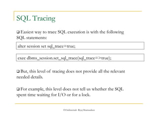

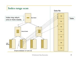
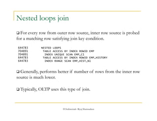
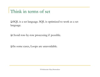
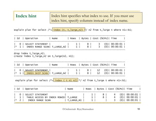
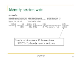
![Simple SELECT
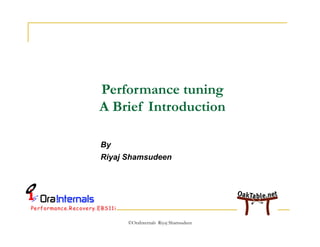
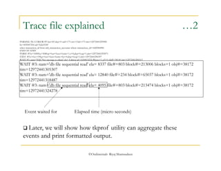
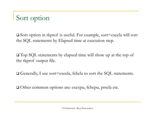
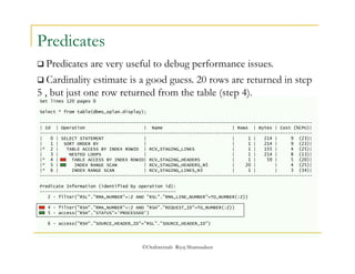
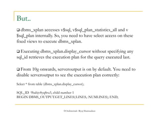
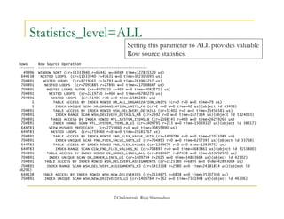
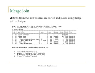
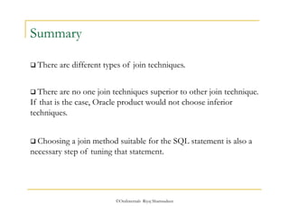
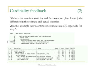
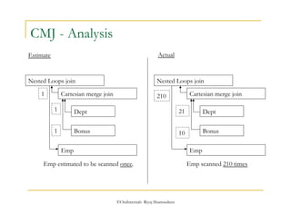
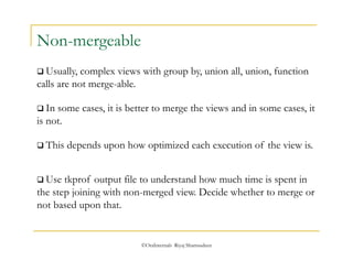
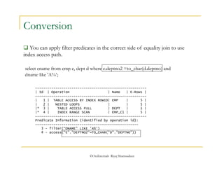
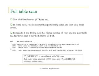
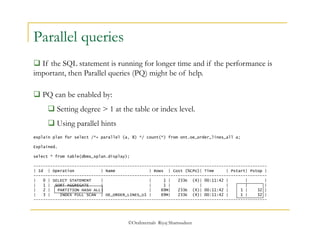
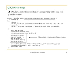
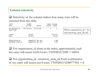
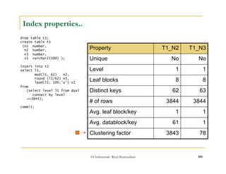
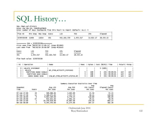
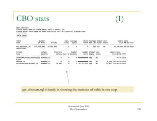
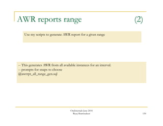
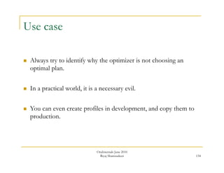
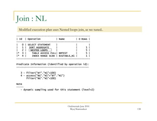
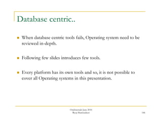
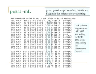
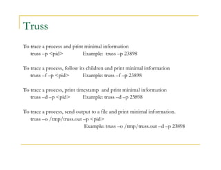
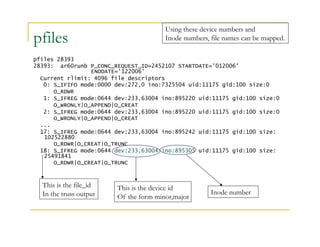
Select * from table(dbms_xplan.display);
--------------------------------------------------------------------------------------
| Id | Operation | Name | Rows | Bytes | Cost (%CPU)| Time |
--------------------------------------------------------------------------------------
| 0 | SELECT STATEMENT | | 975 | 22425 | 512 (1)| 00:00:02 |
|* 1 | HASH JOIN | | 975 | 22425 | 512 (1)| 00:00:02 |
|* 2 | INDEX RANGE SCAN | T2_N1 | 976 | 5856 | 5 (0)| 00:00:01 |
| 3 | TABLE ACCESS BY INDEX ROWID| T1 | 1000 | 17000 | 506 (1)| 00:00:02 |
|* 4 | INDEX RANGE SCAN | T1_N1 | 1000 | | 5 (0)| 00:00:01 |
--------------------------------------------------------------------------------------
Predicate Information (identified by operation id):
---------------------------------------------------
1 - access("T1"."ID"="T2"."ID")
2 - access("T2"."ID"<1000)
4 - access("T1"."ID"<1000)
Execution sequence
(i) Index T2_N1 was scanned with access predicate t2.id <1000 [ Step 2]
(ii) Index T1_N1 was scanned with access predicate t1.id <1000 [ Step 4]
(iii) Table T1 is accessed to retrieve non-indexed column using rowids returned from
©OraInternals Riyaj Shamsudeen
step 2. [ Step 3].
(iv) Rows from step 2 and 3 are joined to create the final result set.[Step 1]](https://image.slidesharecdn.com/performancetuning-aquickintoduction-141006152229-conversion-gate01/85/Performance-tuning-a-quick-intoduction-18-320.jpg)

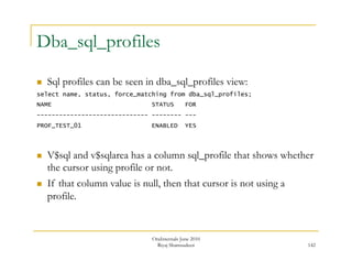
![©OraInternals Riyaj Shamsudeen 89
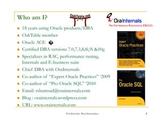
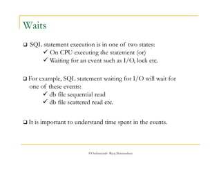
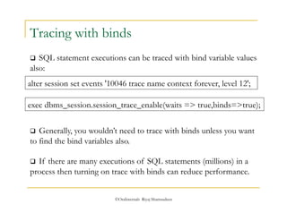
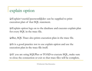
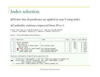
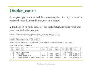
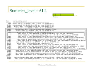
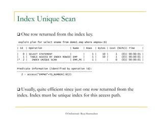
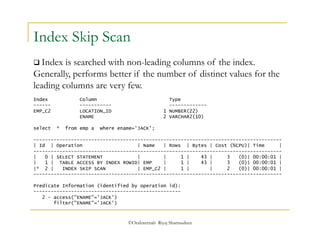
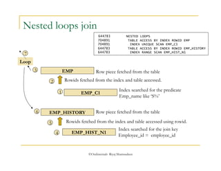
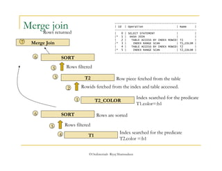
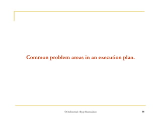
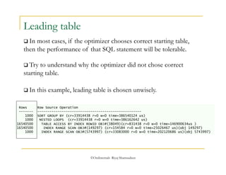
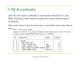
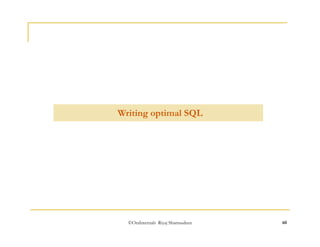
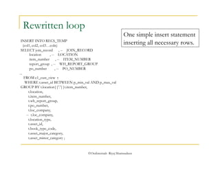
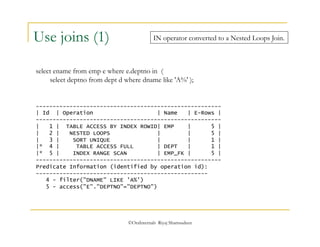
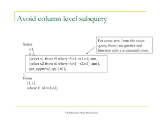
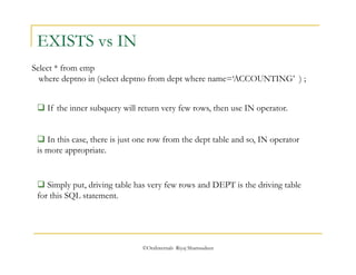
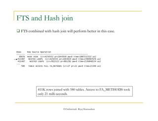
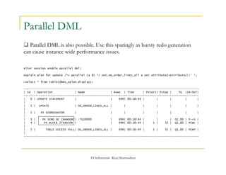
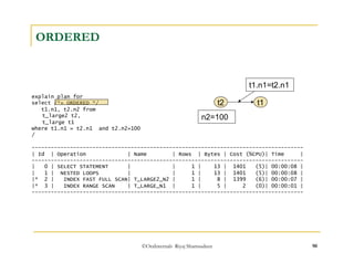
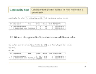
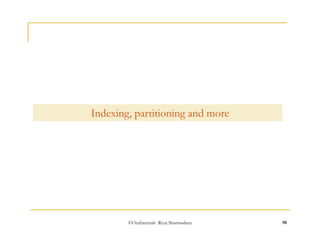
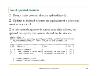
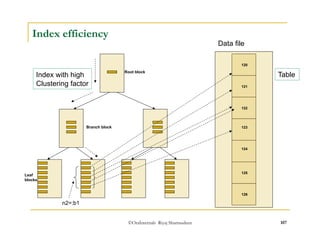
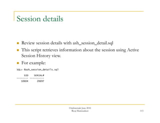
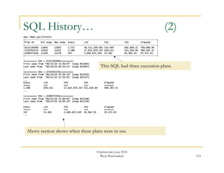
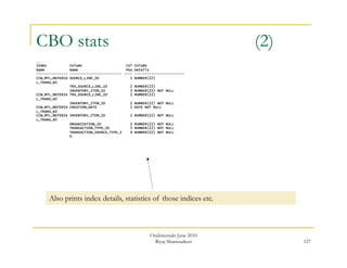
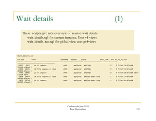
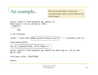
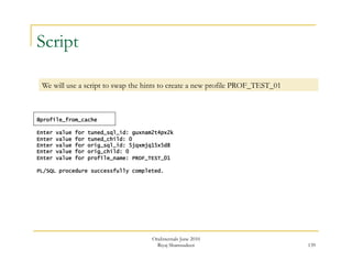
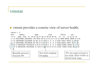
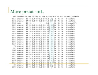
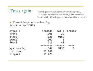
ORDERED
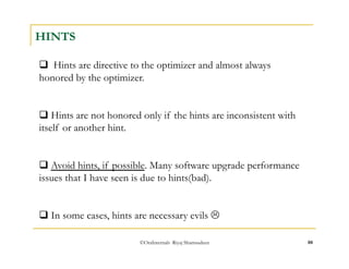
ORDERED hint Dictates optimizer an exact sequence of
tables to join [ top to bottom or L->R canonically speaking].
Select …
From t1,
t2,
t3,
t4
t1 t2 t3 t4](https://image.slidesharecdn.com/performancetuning-aquickintoduction-141006152229-conversion-gate01/85/Performance-tuning-a-quick-intoduction-89-320.jpg)
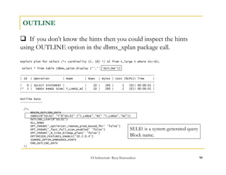
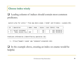
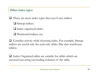

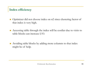
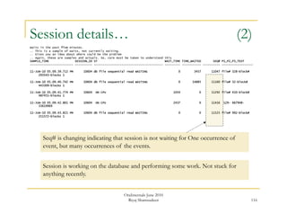
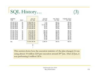
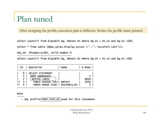
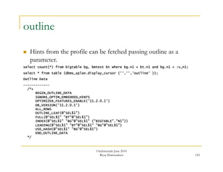

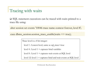
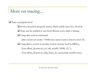
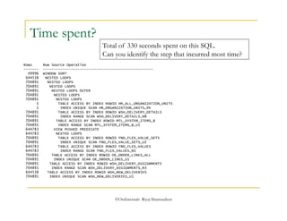
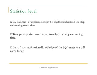
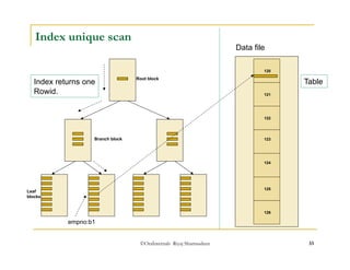
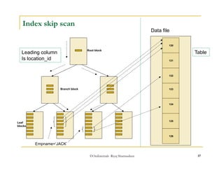
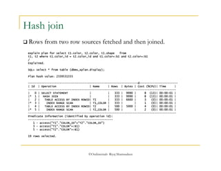
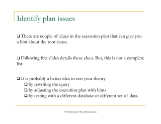
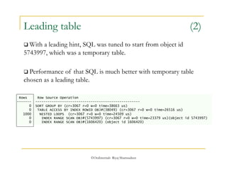
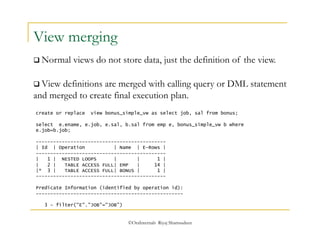
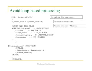
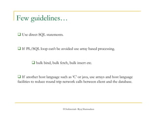
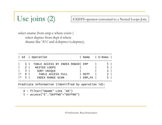
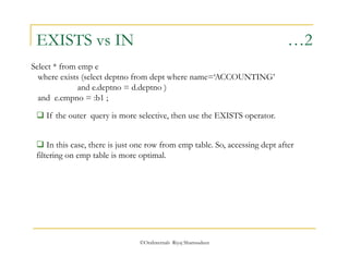
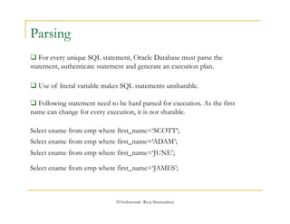
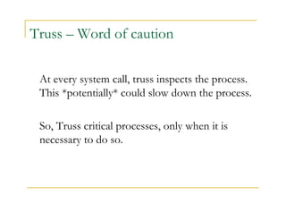
![Truss
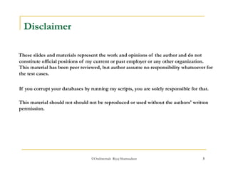
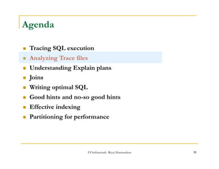
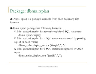
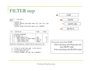
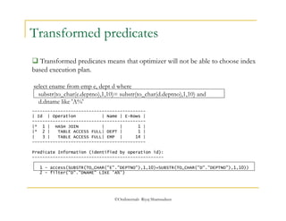
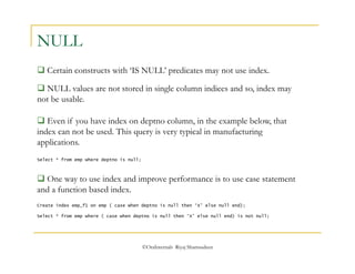
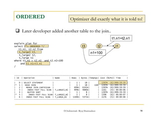
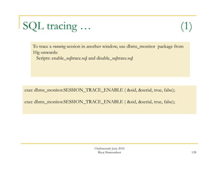
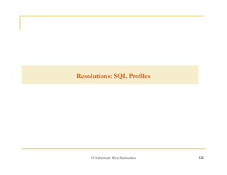
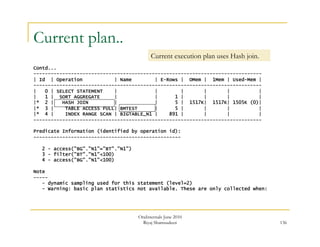
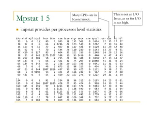
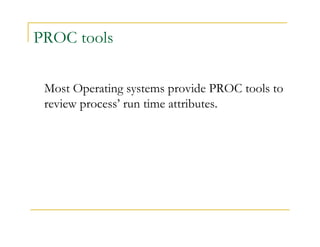
Description:
The truss utility traces the system calls and the signal process receives.
Options:
truss [-fcaeildD] [ - [tTvx] [!] syscall ,...] [ - [sS] [!] signal ,...] [ -
[mM] [!] fault ,...] [ - [rw] [!] fd ,...] [ - [uU] [!] lib ,... : [:] [!] func ,...] [-
o outfile] com- mand | -p pid...
Solaris – truss
Hpux- tusc (download)
Linux – strace](https://image.slidesharecdn.com/performancetuning-aquickintoduction-141006152229-conversion-gate01/85/Performance-tuning-a-quick-intoduction-153-320.jpg)
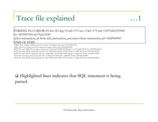
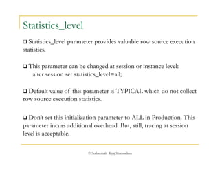
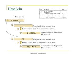
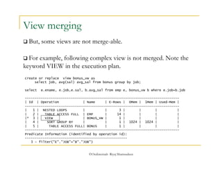
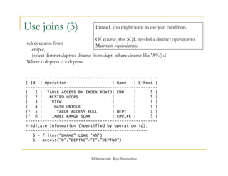
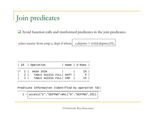
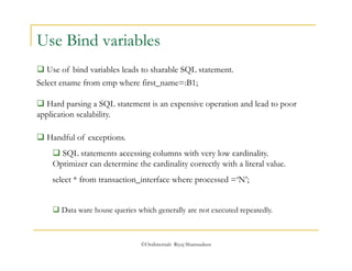
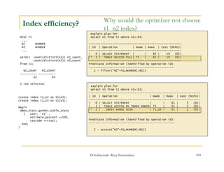
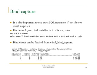
![Truss – Few outputs
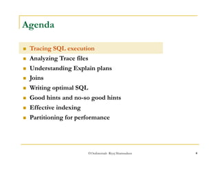
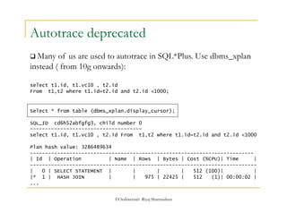
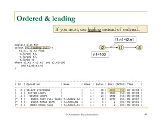
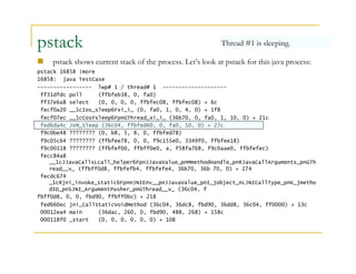
truss -d -o /tmp/truss.out -p 484
cat /tmp/truss.out:
Baase time stamp: 1188872874.8745 [ Mon Sep 3 22:27:54 EDT 2007 ]
0.5942 semtimedop(3735584, 0xFFFFFFFF7FFFDFCC, 1, 0xFFFFFFFF7FFFDFB8) Err#11 EAGAIN
0.5949 ioctl(8, (('7'<<8)|72), 0xFFFFFFFF7FFF87F8) = 192
0.5950 ioctl(8, (('7'<<8)|63), 0x1038AA738) = 0
0.5958 semtimedop(3735584, 0xFFFFFFFF7FFFC26C, 1, 0xFFFFFFFF7FFFC258) = 0
0.5998 ioctl(10, (('V'<<24)|('X'<<16)|('O'<<8)|28), 0xFFFFFFFF7FFFD838) = 0
0.6025 ioctl(10, (('V'<<24)|('X'<<16)|('O'<<8)|28), 0xFFFFFFFF7FFFD838) = 0
0.6047 ioctl(10, (('V'<<24)|('X'<<16)|('O'<<8)|28), 0xFFFFFFFF7FFFD838) = 0
0.6054 ioctl(10, (('V'<<24)|('X'<<16)|('O'<<8)|28), 0xFFFFFFFF7FFFDA48) = 0
0.6059 ioctl(10, (('V'<<24)|('X'<<16)|('O'<<8)|28), 0xFFFFFFFF7FFFD9C8) = 0
0.6064 ioctl(10, (('V'<<24)|('X'<<16)|('O'<<8)|28), 0xFFFFFFFF7FFFD858) = 0
0.6076 ioctl(10, (('V'<<24)|('X'<<16)|('O'<<8)|28), 0xFFFFFFFF7FFFD808) = 0
0.6089 ioctl(10, (('V'<<24)|('X'<<16)|('O'<<8)|28), 0xFFFFFFFF7FFFD8B8) = 0
1.2775 semtimedop(3735584, 0xFFFFFFFF7FFFDFCC, 1, 0xFFFFFFFF7FFFDFB8) = 0
1.2780 ioctl(10, (('V'<<24)|('X'<<16)|('O'<<8)|28), 0xFFFFFFFF7FFF7BF8) = 0
1.2782 ioctl(8, (('7'<<8)|72), 0xFFFFFFFF7FFFA4B8) = 160
1.2783 ioctl(8, (('7'<<8)|63), 0x1038AA738) = 0
1.2785 semtimedop(3735584, 0xFFFFFFFF7FFFD3FC, 1, 0xFFFFFFFF7FFFD3E8) = 0
1.2794 semtimedop(3735584, 0xFFFFFFFF7FFFD3FC, 1, 0xFFFFFFFF7FFFD3E8) = 0
1.2795 ioctl(10, (('V'<<24)|('X'<<16)|('O'<<8)|28), 0xFFFFFFFF7FFFBE08) = 0
1.2797 ioctl(10, (('V'<<24)|('X'<<16)|('O'<<8)|28), 0xFFFFFFFF7FFFBE08) = 0
Time stamp displacement
From base timestamp.
Seconds.fraction of sec](https://image.slidesharecdn.com/performancetuning-aquickintoduction-141006152229-conversion-gate01/85/Performance-tuning-a-quick-intoduction-157-320.jpg)
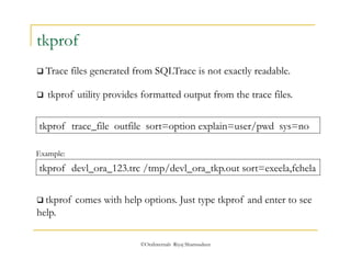
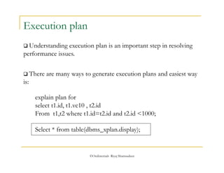
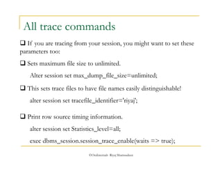
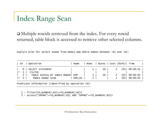
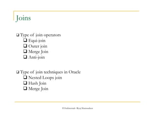
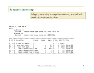
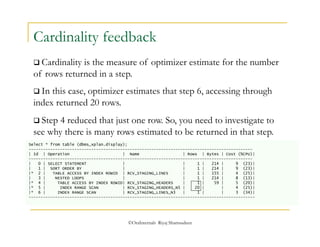
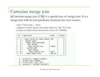
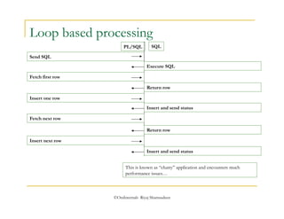
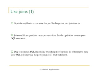
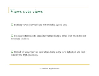
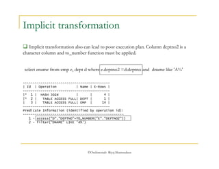
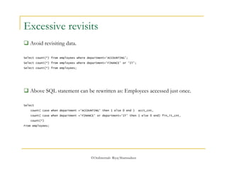
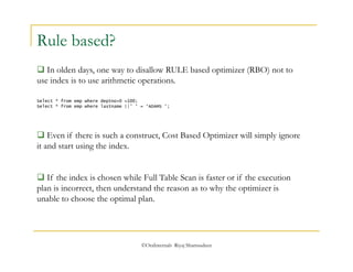
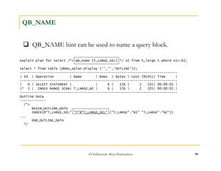
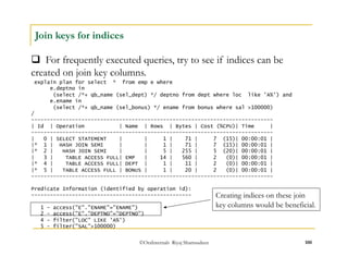
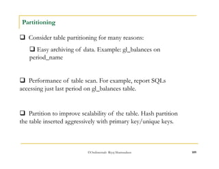
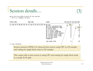
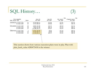
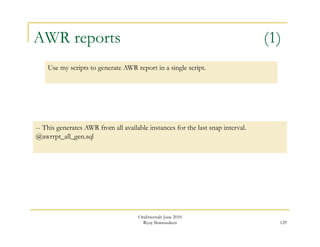
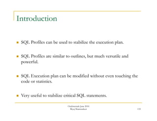
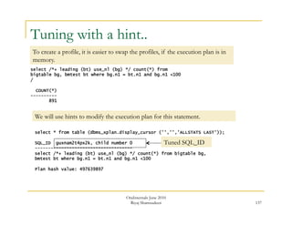
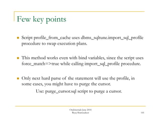
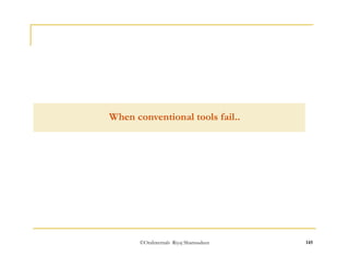
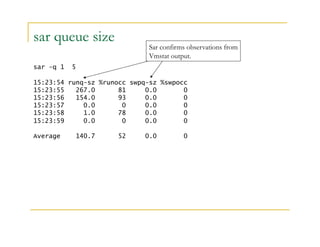
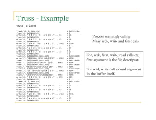
![pmap <pid>
Address Kbytes RSS Anon Locked Mode Mapped File
00010000 72 72 - - r-x-- java
00030000 16 16 16 - rwx-- java
00034000 8744 8680 8680 - rwx-- [ heap ]
77980000 1224 1048 - - r--s- dev:273,2000 ino:104403
77CFA000 24 24 24 - rw--R [ anon ]
77F7A000 24 24 24 - rw--R [ anon ]
78000000 72 72 72 - rwx-- [ anon ]
7814C000 144 144 144 - rwx-- [ anon ]
783E8000 32 32 32 - rwx-- [ anon ]
78408000 8 8 8 - rwx-- [ anon ]
78480000 752 464 - - r--s- dev:85,0 ino:13789
7877E000 8 8 8 - rw--R [ anon ]
78800000 36864 8192 8192 - rwx-- [ anon ]
……
FF25C000 16 8 8 - rwx-- libCrun.so.1
FF276000 8 8 - - rwxs- [ anon ]
FF280000 688 688 - - r-x-- libc.so.1
FF33C000 32 32 32 - rwx-- libc.so.1
FF350000 16 16 16 - rw--- [ anon ]
FF360000 8 8 8 - rwx-- [ anon ]
FF370000 96 96 - - r-x-- libthread.so.1
FF398000 8 8 8 - rwx-- libthread.so.1
FF39A000 8 8 8 - rwx-- libthread.so.1
FF3A0000 8 8 - - r-x-- libc_psr.so.1
FF3B0000 184 184 - - r-x-- ld.so.1
FF3EE000 8 8 8 - rwx-- ld.so.1
FF3F0000 8 8 8 - rwx-- ld.so.1
FF3FA000 8 8 8 - rwx-- libdl.so.1
FFB80000 24 - - - ----- [ anon ]
FFBF0000 64 64 64 - rw--- [ stack ]
-------- ------- ------- ------- -------
total Kb 182352 65568 26360 -
Pmap prints a
Nice memory map
of the Process.
Verious heaps and
Stacks are printed here
Total memory foot print
Also printed.](https://image.slidesharecdn.com/performancetuning-aquickintoduction-141006152229-conversion-gate01/85/Performance-tuning-a-quick-intoduction-161-320.jpg)

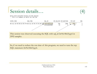
The document provides an introduction to performance tuning. It discusses tracing SQL execution to analyze performance issues. Tracing can be done at different levels, and the tkprof utility helps analyze trace files by providing formatted output. Understanding execution plans is also an important part of performance tuning, as it shows the steps and cost of executing a SQL statement.


![Oracle RAC 12c Practical Performance Management and Tuning OOW13 [CON8825]](https://cdn.slidesharecdn.com/ss_thumbnails/oraclerac12cpracticalperformancemanagementandtuningoow13con8825-131001011452-phpapp01-thumbnail.jpg?width=640&height=640&fit=bounds)


![[Oracle DBA & Developer Day 2012] 高可用性システムに適した管理性と性能を向上させるASM と RMAN の魅力](https://cdn.slidesharecdn.com/ss_thumbnails/ma-4print20121205-200702094006-thumbnail.jpg?width=640&height=640&fit=bounds)


![We Bs Blo Gs Wik Is[1]](https://cdn.slidesharecdn.com/ss_thumbnails/websblogswikis1-100301174146-phpapp02-thumbnail.jpg?width=640&height=640&fit=bounds)