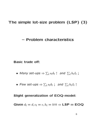
Download to read offline
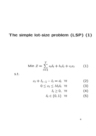
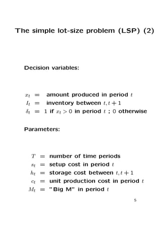
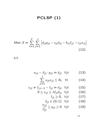
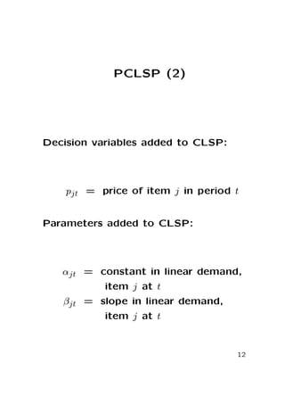
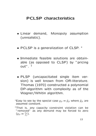
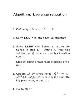
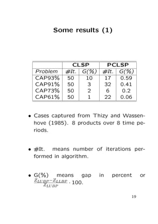
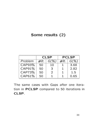
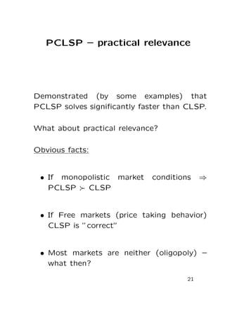

The document introduces the profit maximizing capacitated lot-size problem with pricing (PCLSP) as a generalization of the capacitated lot-sizing problem (CLSP) that allows for pricing decisions. It presents the formulation and characteristics of PCLSP and describes how it is computationally more tractable than CLSP by introducing pricing variables. The document outlines a Lagrange relaxation algorithm for solving PCLSP using lower and upper bound subproblems and presents results showing PCLSP solves faster with smaller optimality gaps than CLSP on example problems. It discusses the practical relevance of PCLSP under different market conditions.