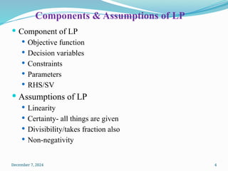
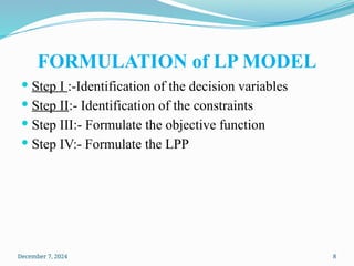
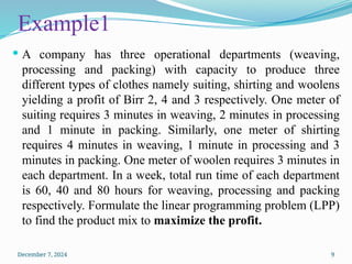
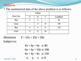
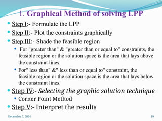
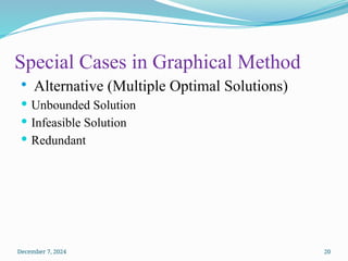
December 7, 2024 1
Linear Programing Problems
***Model Formulation & Graphical
Method***
CHAPTER 2
December 7, 2024 2
Introduction:
 The word linear indicating that all relationships involved
in a particular problem are linear.
 Thus, a given change in one variable will always cause a
resulting proportional change in another variable.
 For example, doubling investment on a certain project
will exactly double the rate of return.
 “Linear programming is a versatile mathematical
technique in O.R and business maths . and a plan of action
to solve a given problem involving linearly related
variables in order to achieve the given objective function
under a given set of constraints.
December 7, 2024 3
Main Application Areas of Linear Programming
Military Applications
Agriculture
Environmental Protection
Facilities Location
Product-Mix
Production
Mixing or Blending
Transportation & Trans-
Shipment
Portfolio Selection
Profit Planning & Contract
Traveling Salesmen
Problem
Media Selection/Evaluation
Staffing
Job analysis
Wages and Salary
Administration.
December 7, 2024 4
Components & Assumptions of LP
 Component of LP
 Objective function
 Decision variables
 Constraints
 Parameters
 RHS/SV
 Assumptions of LP
 Linearity
 Certainty- all things are given
 Divisibility/takes fraction also
 Non-negativity
December 7, 2024 5
Diagrammatically
December 7, 2024 6
Components & Assumptions of LPP
December 7, 2024 7
Advantages & Limitations of LP
 Advantages of LP
 Scientific Approach
 Evaluation of All
Possible Alternatives.
 Quality of Decision
 Flexibility-adaptive/
solves multiple
problems
 Maximum optimal
Utilization of Factors
of Production
 Limitations of LP
 Linear Relationship
 Constant Value of
objective & Constraint
Equations-doesn’t use
probability
 Degree of Complexity
 Multiplicity of Goals
December 7, 2024 8
FORMULATION of LP MODEL
 Step I :-Identification of the decision variables
 Step II:- Identification of the constraints
 Step III:- Formulate the objective function
 Step IV:- Formulate the LPP
December 7, 2024 9
Example1
 A company has three operational departments (weaving,
processing and packing) with capacity to produce three
different types of clothes namely suiting, shirting and woolens
yielding a profit of Birr 2, 4 and 3 respectively. One meter of
suiting requires 3 minutes in weaving, 2 minutes in processing
and 1 minute in packing. Similarly, one meter of shirting
requires 4 minutes in weaving, 1 minute in processing and 3
minutes in packing. One meter of woolen requires 3 minutes in
each department. In a week, total run time of each department
is 60, 40 and 80 hours for weaving, processing and packing
respectively. Formulate the linear programming problem (LPP)
to find the product mix to maximize the profit.
December 7, 2024 10
Solution
 The data can be summarized as follows before
formulating an LPP model.
December 7, 2024 11
 Let x1, x2 and x3 represent the rate of production in the
three departments.
 Maximize Z = 2x1 + 4x2 + 3x3 ……objective function
 Subject to:
 3x1 + 4x2 + 3x3 ≤ 3600 …….. Weaving time constraint
 2x1 + x2 + 3x3 ≤ 2400……. Processing time
constraint
 x1 + 3x2 + 3x3 ≤ 4800 ……. Packing time constraint
 x1 , x2 , x3 ≥ 0. ……. Non-negativity condition
December 7, 2024 12
Example 2
 A small scale manufacturer produces two types of
products A and B which give a profit margin of Birr 4
and Birr 3, respectively. There are two plants I and II,
each having a capability of 72 and 48 hours per day.
Cycle times of A and B are 2 hours and 1 hour in plant
number I, respectively. Similar figures for plant II are 1
and 2 hours. Formulate an LPP model for maximizing the
profit.
December 7, 2024 13
Solutions
 The summarized data of the above problem is as follows:
 Maximize Z = 4x + 3y
Subject to:
2x + y 72
≤
x + 2y 48
≤
x , y 0.
≥
December 7, 2024 14
Example 3
 A firm can produce 3 types of clothes A, B and C.
Three kinds of wools are required with the color of
red, green and blue to produce the clothes. One unit of
A-type cloth consumes 4 meters of red, and 6 meters
of blue wool. One unit of B-type cloth needs 6 meters
of red, 4 meters of green and 4 meters of blue wool.
Type C uses 10 meters of green and 8 meters of blue.
Available stocks are 80, 100 and 150 meters of red,
green and blue wools respectively. Profit margins per
unit of A, B and C are 15, 25 and 20 Birr, respectively.
Formulate an LPP model to maximize the profit.
December 7, 2024 15
Solution
 The summarized data of the above problem is as follows:
Maximize Z = 15x + 25y + 20z
Subject to:
4x + 6y + 0z 80
≤
0x + 4y + 10z 100
≤
6x + 4y + 8z 150
≤
x, y, z 0.
≥
December 7, 2024 16
Example 4
 Demisie Borji and Sons Company is engaged in the
manufacture of three products X, Y and Z. Available data
is given below.
December 7, 2024 17
Solution
 The summarized data of the above problem is as follows:
The LPP Model formulation:
Maximize Z = 10x + 15y + 8z.
Subject to:
x + 2y + 2z ≤ 200
2x + y + z ≤ 220
3x + y + 2z ≤ 180
x , y , z ≥ 0.
December 7, 2024 18
Method for solving LPP
 There are two types of finding a solution for Linear
programming problems.
 Graphic solution and
 Simplex method
December 7, 2024 19
1. Graphical Method of solving LPP
 Step I:- Formulate the LPP
 Step II:- Plot the constraints graphically
 Step III:- Shade the feasible region
 For "greater than" & "greater than or equal to" constraints, the
feasible region or the solution space is the area that lays above
the constraint lines.
 For" less than" &" less than or equal to" constraint, the
feasible region or the solution space is the area that lays below
the constraint lines.
 Step IV:- Selecting the graphic solution technique
 Corner Point Method
 Step V:- Interpret the results
December 7, 2024 20
Special Cases in Graphical Method
 Alternative (Multiple Optimal Solutions)
 Unbounded Solution
 Infeasible Solution
 Redundant

Operational research power point lecture notes

  • 1.
    December 7, 20241 Linear Programing Problems ***Model Formulation & Graphical Method*** CHAPTER 2
  • 2.
    December 7, 20242 Introduction:  The word linear indicating that all relationships involved in a particular problem are linear.  Thus, a given change in one variable will always cause a resulting proportional change in another variable.  For example, doubling investment on a certain project will exactly double the rate of return.  “Linear programming is a versatile mathematical technique in O.R and business maths . and a plan of action to solve a given problem involving linearly related variables in order to achieve the given objective function under a given set of constraints.
  • 3.
    December 7, 20243 Main Application Areas of Linear Programming Military Applications Agriculture Environmental Protection Facilities Location Product-Mix Production Mixing or Blending Transportation & Trans- Shipment Portfolio Selection Profit Planning & Contract Traveling Salesmen Problem Media Selection/Evaluation Staffing Job analysis Wages and Salary Administration.
  • 4.
    December 7, 20244 Components & Assumptions of LP  Component of LP  Objective function  Decision variables  Constraints  Parameters  RHS/SV  Assumptions of LP  Linearity  Certainty- all things are given  Divisibility/takes fraction also  Non-negativity
  • 5.
    December 7, 20245 Diagrammatically
  • 6.
    December 7, 20246 Components & Assumptions of LPP
  • 7.
    December 7, 20247 Advantages & Limitations of LP  Advantages of LP  Scientific Approach  Evaluation of All Possible Alternatives.  Quality of Decision  Flexibility-adaptive/ solves multiple problems  Maximum optimal Utilization of Factors of Production  Limitations of LP  Linear Relationship  Constant Value of objective & Constraint Equations-doesn’t use probability  Degree of Complexity  Multiplicity of Goals
  • 8.
    December 7, 20248 FORMULATION of LP MODEL  Step I :-Identification of the decision variables  Step II:- Identification of the constraints  Step III:- Formulate the objective function  Step IV:- Formulate the LPP
  • 9.
    December 7, 20249 Example1  A company has three operational departments (weaving, processing and packing) with capacity to produce three different types of clothes namely suiting, shirting and woolens yielding a profit of Birr 2, 4 and 3 respectively. One meter of suiting requires 3 minutes in weaving, 2 minutes in processing and 1 minute in packing. Similarly, one meter of shirting requires 4 minutes in weaving, 1 minute in processing and 3 minutes in packing. One meter of woolen requires 3 minutes in each department. In a week, total run time of each department is 60, 40 and 80 hours for weaving, processing and packing respectively. Formulate the linear programming problem (LPP) to find the product mix to maximize the profit.
  • 10.
    December 7, 202410 Solution  The data can be summarized as follows before formulating an LPP model.
  • 11.
    December 7, 202411  Let x1, x2 and x3 represent the rate of production in the three departments.  Maximize Z = 2x1 + 4x2 + 3x3 ……objective function  Subject to:  3x1 + 4x2 + 3x3 ≤ 3600 …….. Weaving time constraint  2x1 + x2 + 3x3 ≤ 2400……. Processing time constraint  x1 + 3x2 + 3x3 ≤ 4800 ……. Packing time constraint  x1 , x2 , x3 ≥ 0. ……. Non-negativity condition
  • 12.
    December 7, 202412 Example 2  A small scale manufacturer produces two types of products A and B which give a profit margin of Birr 4 and Birr 3, respectively. There are two plants I and II, each having a capability of 72 and 48 hours per day. Cycle times of A and B are 2 hours and 1 hour in plant number I, respectively. Similar figures for plant II are 1 and 2 hours. Formulate an LPP model for maximizing the profit.
  • 13.
    December 7, 202413 Solutions  The summarized data of the above problem is as follows:  Maximize Z = 4x + 3y Subject to: 2x + y 72 ≤ x + 2y 48 ≤ x , y 0. ≥
  • 14.
    December 7, 202414 Example 3  A firm can produce 3 types of clothes A, B and C. Three kinds of wools are required with the color of red, green and blue to produce the clothes. One unit of A-type cloth consumes 4 meters of red, and 6 meters of blue wool. One unit of B-type cloth needs 6 meters of red, 4 meters of green and 4 meters of blue wool. Type C uses 10 meters of green and 8 meters of blue. Available stocks are 80, 100 and 150 meters of red, green and blue wools respectively. Profit margins per unit of A, B and C are 15, 25 and 20 Birr, respectively. Formulate an LPP model to maximize the profit.
  • 15.
    December 7, 202415 Solution  The summarized data of the above problem is as follows: Maximize Z = 15x + 25y + 20z Subject to: 4x + 6y + 0z 80 ≤ 0x + 4y + 10z 100 ≤ 6x + 4y + 8z 150 ≤ x, y, z 0. ≥
  • 16.
    December 7, 202416 Example 4  Demisie Borji and Sons Company is engaged in the manufacture of three products X, Y and Z. Available data is given below.
  • 17.
    December 7, 202417 Solution  The summarized data of the above problem is as follows: The LPP Model formulation: Maximize Z = 10x + 15y + 8z. Subject to: x + 2y + 2z ≤ 200 2x + y + z ≤ 220 3x + y + 2z ≤ 180 x , y , z ≥ 0.
  • 18.
    December 7, 202418 Method for solving LPP  There are two types of finding a solution for Linear programming problems.  Graphic solution and  Simplex method
  • 19.
    December 7, 202419 1. Graphical Method of solving LPP  Step I:- Formulate the LPP  Step II:- Plot the constraints graphically  Step III:- Shade the feasible region  For "greater than" & "greater than or equal to" constraints, the feasible region or the solution space is the area that lays above the constraint lines.  For" less than" &" less than or equal to" constraint, the feasible region or the solution space is the area that lays below the constraint lines.  Step IV:- Selecting the graphic solution technique  Corner Point Method  Step V:- Interpret the results
  • 20.
    December 7, 202420 Special Cases in Graphical Method  Alternative (Multiple Optimal Solutions)  Unbounded Solution  Infeasible Solution  Redundant