Download to read offline
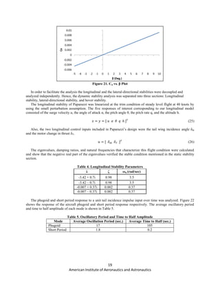
![11
American Institute of Aeronautics and Astronautics
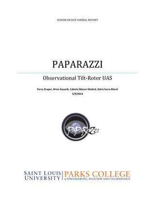
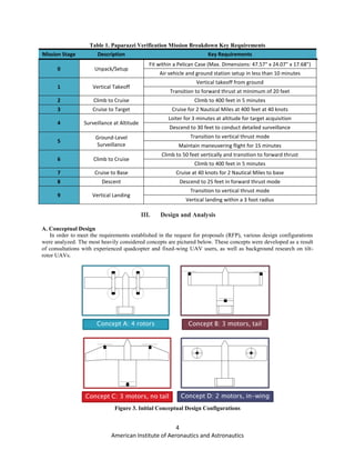
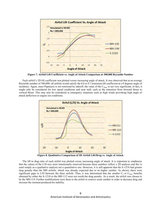
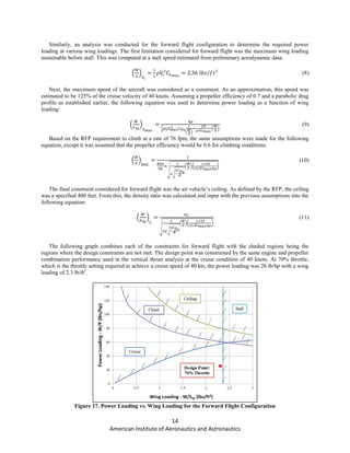
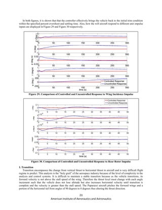
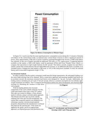
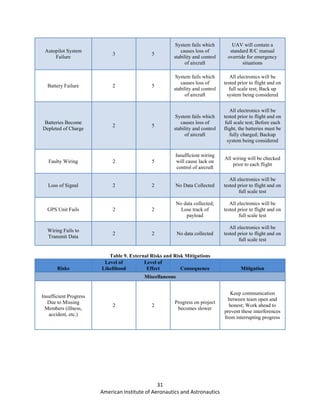
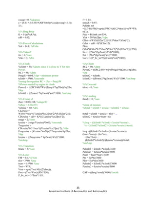
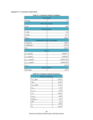
Figure 13. Paparazzi Aircraft Dimensions
A tool was developed in Excel to estimate the drag of the UAS based on a buildup of the system’s various
components using Shevell’s method. This calculates the entire system drag by summing the drag of each of the
system’s structures, according to the equation:
∑ (2)
Where K is defined as,
[ ( ) ( ) ]
( ) ⁄
√ ⁄
(3)
The skin friction coefficient was calculated using a simplified assumption of entirely turbulent flow. It was
assumed that the flow was tripped to turbulent flow at .01 inches on each component. The summed components of
the plane include the rectangular portion of the wing, the engine nacelles, the fuselage, and the tail. With the given
dimensions specified in Table 3, a Reynolds number was calculated for each surface of the aircraft.
Table 3. Freestream Parameters
Pressure (psf) 2051
Density (lbs./ft2
) 2.32E-03
Velocity (ft/s) 67.5
Viscosity (lb ft-1
s-1
) 3.73E-07
Mach Number (M) 0.06
Speed of Sound (ft/s) 1113
Dynamic Pressure (psf) 5.28](https://image.slidesharecdn.com/b6d5ca9f-0cd8-4fef-be65-ca3bfedf9c4c-151130202313-lva1-app6891/85/Paparrazzi_Final-1-12-320.jpg)
![13
American Institute of Aeronautics and Astronautics
provide enough thrust in horizontal flight to reach the cruise speed. For efficiency in vertical thrust mode a propeller
with large diameter and low pitch is desired as opposed to horizontal thrust where low diameter and higher pitch is
ideal. By analyzing different propeller combinations with our motor in MotoCalc, software commonly used to
predict RC aircraft performance, a propeller that is 12”x8” was selected. This offers the minimum thrust with this
motor needed to reach the cruise speed of 40 knots while having the largest diameter and lowest pitch possible for
the highest efficiency during vertical thrust.
F. Constraint Analysis
An initial constraint analysis tool was developed in Excel with estimated data and then adjusted iteratively as
various design assumptions became more strongly defined. As aircraft and helicopter designs are constrained by
separate parameters, the analysis had to consider the vertical thrust configuration and the forward configuration
constraints separately. Primarily, the limiting values for helicopter takeoff and hovering is power loading and disk
loading. For an aircraft, these values would be power loading and wing loading. While the power loading constraint
is inherently related, each configuration will use a separate throttle setting which will consequently affect the power
required.
The following equation was used to determine the power required for vertical climb at various disk loadings out
of ground effect:
[( √ ) ] [ ] (7)
It should be noted that this equation also applies for hovering flight by setting the climb velocity to zero.
Intuitively, it also becomes apparent that the air vehicle will have enough power to hover if the vehicle has the
power required for climb. Therefore, a climb rate of 120 fpm was assumed to allow the air vehicle to reach an
altitude of 20 feet in 10 seconds. The adjustment for the force of downwash blowing on the vehicle was assumed to
be 3% of the disk loading. Additionally, the figure of merit was assumed to be 0.7 to compensate power losses due
to factors such as airfoil profile drag, nonuniform flow, tip losses, and slipstream effects. The mechanical efficiency
was approximated to be 0.97. Although this analysis considers the power required out of ground effect, the actual
power required during takeoff in ground effect is decreased. However, in an effort to design with conservative
assumptions and allow excess power for maneuvering, ground effect was neglected for power calculations.
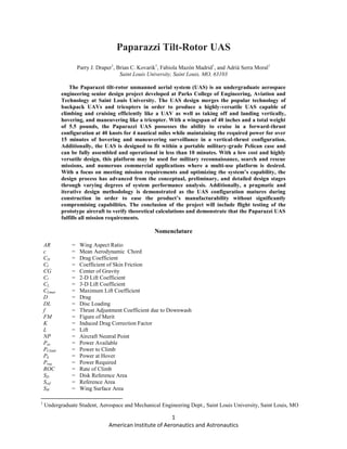
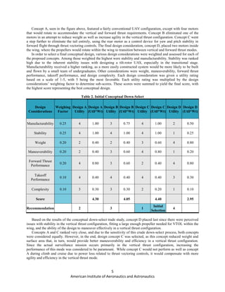
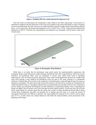
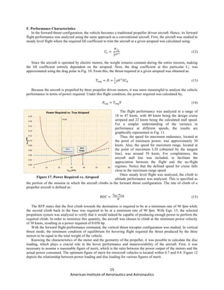
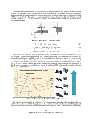
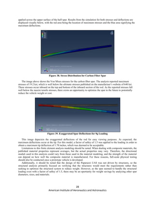
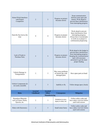
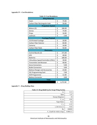
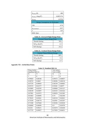
Using an assumed weight of 5.50 lbs, the power loading was plotted versus the disk loading. In the figure below,
the area above the curve represents an inoperable region, where there is not sufficient power to takeoff at 120 fpm.
The area below the curve is the design space which meets VTOL power requirements. The design point for climb
was selected to be a power loading of 5.7 lbs/hp at a disk loading of 7.0 lbs/ft2
. With the current engine and propeller
combination, this occurs at an 80% throttle setting, which is the upper limit for our desired maneuvering mission.
With the design point falling beneath the curve, there is a surplus of power available as a margin of safety which
could also be used to accelerate the vehicle upwards at a greater rate if required during takeoff or maneuvering
flight.
Figure 16. Power Loading vs. Disk Loading for the Vertical Thrust Configuration](https://image.slidesharecdn.com/b6d5ca9f-0cd8-4fef-be65-ca3bfedf9c4c-151130202313-lva1-app6891/85/Paparrazzi_Final-1-14-320.jpg)
![16
American Institute of Aeronautics and Astronautics
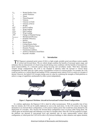
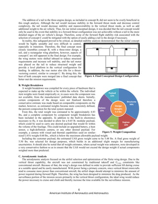
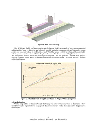
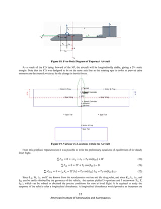
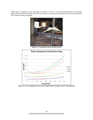
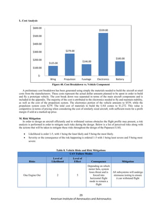
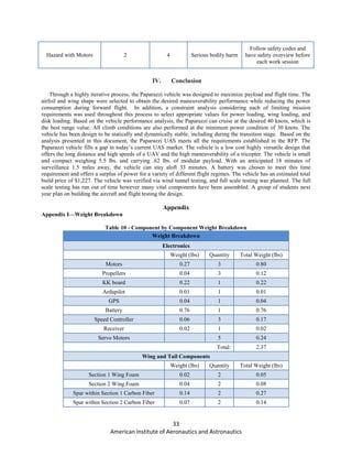
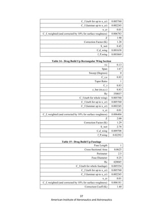
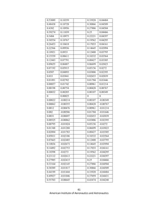
The optimum figure of merit of the Paparazzi
UAS was assumed to be the minimum optimal value
of 0.7 in order to be conservative and allow extra
room in possible losses or future changes in the
design which might have an effect on the overall
performance of the vehicle. Once the figure of merit
was defined, the power requirements to takeoff and
hover were calculated. The disk loading required to
hover was estimated to be 2.33 psf, and it was
determined that each motor had to produce 0.106 hp
to hover, resulting in a total power required of 0.351
hp. Note that an extra 10% was added to the total
power result in order to account for potential drag
and transmission losses.
Since the power required to hover is a
representation of the minimum amount of power
required to maintain the UAS in a fixed equilibrium
position with the environment, the power required to
climb was estimated by using the conservation of energy relationship.
(16)
[ √( ) ] (17)
Then, to find the total power required to climb to the minimum transition height of 20 feet, it was necessary to
assume a suitable Vc of 180 fpm, and the total power required to takeoff was computed to be 0.42 hp.
H. Stability
The first approach towards determining the stability conditions of the aircraft was followed by making a more
precise estimation of the center of gravity’s location. In order to find the location of the CG, every component
included in the vehicle was considered as a point mass with a defined weight and location; then, the CG equation
yielded,
∑ ∑
(18)
In order to use the equation above, the point mass locations of the wings, fuselage, tail, and spars were found by
calculating the moment of area of the surfaces and dividing by its mass:
(19)
From the equations above, the CG location was calculated to be 4.0 inches from the leading edge. This was set
constant to be at the location of rotation for transition. From the aerodynamic analysis the wing’s aerodynamic
center was found to be located 4.36 inches aft the rectangular section leading edge as computed. A 2D
representation of the location of each point mass, the CG location, and the NP location was developed as a visual
representation.
Figure 18. Power and Disc Loading for Figures of Merit](https://image.slidesharecdn.com/b6d5ca9f-0cd8-4fef-be65-ca3bfedf9c4c-151130202313-lva1-app6891/85/Paparrazzi_Final-1-17-320.jpg)
![42
American Institute of Aeronautics and Astronautics
0.61454 -0.00262 0.5 -0.03978
0.671 0.00085 0.56526 -0.03638
0.72557 0.00378 0.62941 -0.03247
0.77737 0.00601 0.69134 -0.02823
0.82556 0.00742 0.75 -0.02384
0.86933 0.00793 0.80438 -0.01945
0.90792 0.00757 0.85355 -0.01522
0.94063 0.00634 0.89668 -0.01127
0.96666 0.00442 0.93301 -0.0077
0.9853 0.0023 0.96194 -0.00463
0.99635 0.00063 0.98296 -0.00218
1 0 0.99572 -0.00057
1 0
Appendix VIII—Wind Tunnel Data Reduction
%% Wind Tunnel Analysis
%Team Paparazzi
clear
clc
%% Conversion Factors
% < < Distance > >
nm_2_miles = 1.15078; %multiply to convert from nm to miles
miles_2_ft = 5280; %multiply to convert from miles to feet
in_2_ft = 1/12; %multiply to convert from in to ft
% < < Speed > >
kts_2_mph = 1.1508; %multiply to convert from kts to mph
kts_2_fps = 1.6878; %multiply to convert from kts to fps
mph_2_fps = 1.46667; %multiply to convert from mph to fps
% < < Mass > >
oz_2_lbs = 1/16; %multiply to convert from oz to lbs
% < < Temperature > >
fah_2_rank = 460.67; %add to convert from Fahrenheit to Rankine
% < < Pressure > >
inHg_2_psf = 70.7262; %multiply to convert from inches Mercury
to Psf
% < < Time > >
hour_2_sec = 3600; %multiply to convert from hours to seconds
min_2_sec = 60; %multiply to convert from min to seconds
% < < Angles > >
deg_2_rad = pi/180; %multiply to convert from degrees to radians
%% Atmospheric Conditions
Tatm = 76; %Fahrenheit
Tatm = Tatm + fah_2_rank; %Convert to working units
Patm = 29.5; %inches of Mercury
Patm = Patm*inHg_2_psf; %Convert to working units
Rair = 1716; %Air Constant in engineering units
Density = Patm/(Rair*Tatm); %Air Density at Given Conditions
mu = (3.62*10^-
7)*((Tatm/518.7)^1.5)*((518.7+198.72)/(Tatm+198.72));
%air viscocity in engineering units at Patm and Tatm
%-> Got equation from Introduction to Flight 7th ed.
nu = mu/Density;
a_SL = 1116; %Speed of Sound at SL in fps
%% Chosen Testing Variables
Vvec = [0 15 20 25 30 35 40 45 60 92]; %Wind Tunnel Speeds in
mph
Vvec = Vvec*mph_2_fps; %Convert to working units
q_s = 0.5*Density*Vvec.^2; %Uncorrected Dynamic Pressure
Vector
%% Wind Tunnel Test Section Geometry
H = 28; %Test Section Height in inches
H = H*in_2_ft; %Convert to working units
B = 40; %Test Section Width in inches
B = B*in_2_ft; %Convert to working units
Lts = 54; %Test Section Length in inches
Lts = Lts*in_2_ft; %Convert to working units
Acs = H*B; %Test Section Cross-sectional (Frontal) Area
Ats = H*Lts; %Test Section Area
Strut_D = 1.5; %Strut Diameter in inches <<NOT UPDATED>>
Strut_D = Strut_D*in_2_ft; %Convert to working units
Strut_L = 15; %Strut Length in inches <<NOT UPDATED>>](https://image.slidesharecdn.com/b6d5ca9f-0cd8-4fef-be65-ca3bfedf9c4c-151130202313-lva1-app6891/85/Paparrazzi_Final-1-43-320.jpg)
![43
American Institute of Aeronautics and Astronautics
Strut_L = Strut_L*in_2_ft; %Convert to working units
Astrut = Strut_D*Strut_L; %THis is the Area in contact with free
stream
%% Paparazzi Aircraft Wind Tunnel Model Geometry
% < < Wing > >
bw = 20; %Wing Span in inches
bw = bw*in_2_ft; %Convert to working units
cbar_w = 4.25; %Wing MAC in inches
cbar_w = cbar_w*in_2_ft; %Convert to working units
Sw = bw*cbar_w; %Wing Area
ARw = (bw^2)/Sw; %Wing Aspect Ratio
Vol_w = 31.29; %Wing Volume in inches cube
Vol_w = Vol_w*(in_2_ft^3); %Convert to working units
X_CG = 2; %CG location from wing LE in inches
X_CG = X_CG*in_2_ft; %Convert to working units
tw = 0.1305*cbar_w; %Wing Thickness
Rew = (Vvec*cbar_w)/nu; %Wing Reynolds Number Vector
% < < Tail > >
bt = 10.63; %Tail Span in inches
bt = bt*in_2_ft; %Convert to working units
cbar_t = 3.25; %Tail MAC in inches
cbar_t = cbar_t*in_2_ft; %Convert to working units
St = bt*cbar_t; %Tail Area
ARt = (bt^2)/St; %Tail Aspect Ratio
lt = 7.5; %Distance from CG to Tail Aerodynamic Center (@ c/4)
in inches
lt = lt*in_2_ft; %Convert to working units
V_H = (lt*St)/(cbar_w*Sw); %Tail Volume Coefficient
Ret = (Vvec*cbar_t)/nu; %Tail Reynolds Number Vector
% < < Fuselage > >
Vol_f = 7.4668; %Fuselage Volume in inches cube
Vol_f = Vol_f*(in_2_ft^3); %Convert to working units
X_balance_CG = 0.94; %X-Distance between Balance and
Aircraft CG in inches
X_balance_CG = X_balance_CG*in_2_ft; %Convert to working
units
Z_balance_CG = 0.50; %Z-Distance between Balance and Aircraft
CG in inches
Z_balance_CG = Z_balance_CG*in_2_ft; %Convert to working
units
D_f = 1.5; %Fuselage Diameter in inches
D_f = D_f*in_2_ft; %Convert to working units
L_f = 6.875; %Fuselage Length in inches
L_f = L_f*in_2_ft; %Convert to working units
%% Figure Parameters
% < < Figure 6.23 > >
% Read from ARw and Taper Ratio = 1
bv_b = 0.86; %Get
% < < Figure 6.29 > >
bv = bv_b*bw;
be = (bw + bv)*0.5;
K = be/B;
be_B = be/B; %Read and Taper Ratio = 1
Delta = 0.146; %Get
% < < Figure 6.52 > >
lt_B = lt/B; %Read and Taper Ratio = 1
Tau2 = 0.35; %Get
% < < Figure 6.13 > >
tw_cbarw = tw/cbar_w; %Read (Airfoil not in the chart,
approximated)
Df_Lf = D_f/L_f; %Read
K1 = 0.997; %Get
K3 = 0.95; %Get
% < < Figure 6.14 > >
b2_B = 2*bw/B; %Read
B_H = B/H; %Read
Tau1 = 0.9125; %Get
%% Constant Correction Coefficients
Esbw = (K1*Tau1*Vol_w)/(Acs^(3/2));
EsbB = (K3*Tau1*Vol_f)/(Acs^(3/2));
Esbt = Esbw+EsbB;
Estrut_windshield = 0.25*(Acs/Ats);
DCmcg_Ddelta = -0.0626*V_H; %Assuming
%% Wind Tunnel Test
%% No Wind with Model Data
%import .dat file to matlab
[Data,SizeData] = importfile('no_wind.dat', 2);
%Substract First Row which to substract Zero offset error](https://image.slidesharecdn.com/b6d5ca9f-0cd8-4fef-be65-ca3bfedf9c4c-151130202313-lva1-app6891/85/Paparrazzi_Final-1-44-320.jpg)
![44
American Institute of Aeronautics and Astronautics
for i = 2:1:SizeData(1)
Data(i,:) = Data(i,:) - Data(1,:);
end
alpha_no_wind = Data(2:end,1); %AoA vector in Deg.
Lift_no_wind = Data(2:end,2); %Lift Vector in lbs.
Drag_no_wind = Data(2:end,3); %Drag Vector in lbs.
Pitch_no_wind = Data(2:end,4)*in_2_ft; %Pitching Moment
Vector in lbs*ft
Side_no_wind = Data(2:end,5); %Sideforce Vector in lbs
Roll_no_wind = Data(2:end,6)*in_2_ft; %Rolling Moment Vector
in lbs*ft
Yaw_no_wind = Data(2:end,7)*in_2_ft; %Yawing Moment
Vector in lbs*ft
%% No Model with Wind at 92 mph Data
%import .dat file to matlab
[Data]= importfile('no_model_92mph.dat', 2);
alpha_no_model_92mph = Data(1:end,1); %AoA vector in Deg.
Lift_no_model_92mph = Data(1:end,2); %Lift Vector in lbs.
Drag_no_model_92mph = Data(1:end,3); %Drag Vector in lbs.
Pitch_no_model_92mph = Data(1:end,4)*in_2_ft; %Pitching
Moment Vector in lbs*ft
Side_no_model_92mph = Data(1:end,5); %Sideforce Vector in lbs
Roll_no_model_92mph = Data(1:end,6)*in_2_ft; %Rolling
Moment Vector in lbs*ft
Yaw_no_model_92mph = Data(1:end,7)*in_2_ft; %Yawing
Moment Vector in lbs*ft
%To correct Cruise conditions besides 92 mph, we need to
nondimensionalize the Data
%Divide Loads by 0.5*Density*V^2*Sstruts
%Divide Moments by 0.5*Density*V^2*Sstruts*Dstrut
CLs_no_model =
Lift_no_model_92mph/(0.5*Density*(Vvec(end)^2)*Astrut);
CDs_no_model =
Drag_no_model_92mph/(0.5*Density*(Vvec(end)^2)*Astrut);
CSFs_no_model =
Side_no_model_92mph/(0.5*Density*(Vvec(end)^2)*Astrut);
CMs_no_model =
Pitch_no_model_92mph/(0.5*Density*(Vvec(end)^2)*Astrut*Stru
t_D);
CLRs_no_model =
Roll_no_model_92mph/(0.5*Density*(Vvec(end)^2)*Astrut*Strut
_D);
CNs_no_model =
Yaw_no_model_92mph/(0.5*Density*(Vvec(end)^2)*Astrut*Strut
_D);
%% Cruise Analysis:
%% < < Speed = 30 mph > >
%import .dat file to matlab
[Data,SizeData] = importfile('cruise_30mph.dat', 2);
%Substract First Row which to substract Zero offset error
for i = 2:1:SizeData(1)
Data(i,:) = Data(i,:) - Data(1,:);
end
alpha_cruise_30mph = Data(2:end,1); %AoA vector in Deg.
Lift_cruise_30mph = Data(2:end,2); %Lift Vector in lbs.
Drag_cruise_30mph = Data(2:end,3); %Drag Vector in lbs.
Pitch_cruise_30mph = Data(2:end,4)*in_2_ft; %Pitching Moment
Vector in lbs*ft
Side_cruise_30mph = Data(2:end,5); %Sideforce Vector in lbs
Roll_cruise_30mph = Data(2:end,6)*in_2_ft; %Rolling Moment
Vector in lbs*ft
Yaw_cruise_30mph = Data(2:end,7)*in_2_ft; %Yawing Moment
Vector in lbs*ft
%First, we correct for no wind effect
Lift_cruise_30mph_corr = Lift_cruise_30mph - Lift_no_wind;
Drag_cruise_30mph_corr = Drag_cruise_30mph - Drag_no_wind;
Pitch_cruise_30mph_corr = Pitch_cruise_30mph - Pitch_no_wind;
Side_cruise_30mph_corr = Side_cruise_30mph - Side_no_wind;
Roll_cruise_30mph_corr = Roll_cruise_30mph - Roll_no_wind;
Yaw_cruise_30mph_corr = Yaw_cruise_30mph - Yaw_no_wind;
%Now, Since V is not 92 mph, we nondimensionalize Lift and
Drag
%To correct for no model in Lift and Drag to find other correction
factors
CLs_cruise_30mph_corr =
Lift_cruise_30mph_corr/(0.5*Density*(Vvec(5)^2)*Sw);
CDs_cruise_30mph_corr =
Drag_cruise_30mph_corr/(0.5*Density*(Vvec(5)^2)*Sw);
%Now we correct for no model error
CLs_cruise_30mph_corr = CLs_cruise_30mph_corr -
CLs_no_model;
CDs_cruise_30mph_corr = CDs_cruise_30mph_corr -
CDs_no_model;
%Now we compute CL squared to find K and CD0
CLs_cruise_30mph_CG_sq = CLs_cruise_30mph_corr.^2;
%{
%We plot to have a sense of the results (Should be a straigth line)
figure
plot(CLs_cruise_30mph_CG_sq,CDs_cruise_30mph_corr)
%}
%We do a linear fit to compute the slope and the CD intercept
(CD0)
CL_sq_CD_30mph_Eq =
polyfit(CLs_cruise_30mph_CG_sq,CDs_cruise_30mph_corr,1);
%Compute K
K_cruise_30mph = CL_sq_CD_30mph_Eq(1);
%Compute e
e_osw_cruise_30mph = 1/(K_cruise_30mph*ARw*pi);
%Compute CD0
CD0_cruise_30mph = CL_sq_CD_30mph_Eq(2);
%Find Missing correction factors
Ewbt_cruise_30mph = (Sw/(4*Acs))*CD0_cruise_30mph;
Etot_cruise_30mph = Esbt + Ewbt_cruise_30mph +
Estrut_windshield;
%Compute Corrected dynamic pressure
q_corr_cruise_30mph = q_s(5)*(1+Etot_cruise_30mph)^2;
%Use Corrected dynamic pressure to compute all coefficients
CLs_cruise_30mph_corr =
Lift_cruise_30mph_corr/(q_corr_cruise_30mph*Sw);
CDs_cruise_30mph_corr =
Drag_cruise_30mph_corr/(q_corr_cruise_30mph*Sw);](https://image.slidesharecdn.com/b6d5ca9f-0cd8-4fef-be65-ca3bfedf9c4c-151130202313-lva1-app6891/85/Paparrazzi_Final-1-45-320.jpg)
![45
American Institute of Aeronautics and Astronautics
CSFs_cruise_30mph_corr =
Side_cruise_30mph_corr/(q_corr_cruise_30mph*Sw);
CMs_cruise_30mph_corr =
Pitch_cruise_30mph_corr/(q_corr_cruise_30mph*Sw*cbar_w);
CLRs_cruise_30mph_corr =
Roll_cruise_30mph_corr/(q_corr_cruise_30mph*Sw*cbar_w);
CNs_cruise_30mph_corr =
Yaw_cruise_30mph_corr/(q_corr_cruise_30mph*Sw*cbar_w);
%Now we correct all coefficients for no model error
CLs_cruise_30mph_corr = CLs_cruise_30mph_corr -
CLs_no_model;
CDs_cruise_30mph_corr = CDs_cruise_30mph_corr -
CDs_no_model;
CSFs_cruise_30mph_corr = CSFs_cruise_30mph_corr -
CSFs_no_model;
CMs_cruise_30mph_corr = CMs_cruise_30mph_corr -
CMs_no_model;
CLRs_cruise_30mph_corr = CLRs_cruise_30mph_corr -
CLRs_no_model;
CNs_cruise_30mph_corr = CNs_cruise_30mph_corr -
CNs_no_model;
%Compute AoA correction Vector
Delta_alpha_cruise_30mph =
Delta*(1+Tau2)*(Sw/Acs)*(180/pi)*CLs_cruise_30mph_corr;
%Corrected AoA
alpha_cruise_30mph_corr = alpha_cruise_30mph +
Delta_alpha_cruise_30mph;
%Drag Wall Correction
Delta_Cd_cruise_30mph =
Delta*(Sw/Acs)*(CLs_cruise_30mph_corr.^2);
%Tail Moment Coefficient Correction Vector
Delta_Cm_CG_cruise_30mph =
DCmcg_Ddelta*(Sw/Acs)*(180/pi)*Delta*Tau2*...
CLs_cruise_30mph_corr;
%Now we translate the Loads and moments from Balance Center
to CG
%Loads_CG = Loads_Balance
%Moments_CG = Moment_Balance +- Loads*distance
CLs_cruise_30mph_corr_CG = CLs_cruise_30mph_corr;
CDs_cruise_30mph_corr_CG = CDs_cruise_30mph_corr +
Delta_Cd_cruise_30mph;
CSFs_cruise_30mph_corr_CG = CSFs_cruise_30mph_corr;
CMs_cruise_30mph_corr_CG = (CMs_cruise_30mph_corr +...
CLs_cruise_30mph_corr*(X_balance_CG/cbar_w)-...
CDs_cruise_30mph_corr*(Z_balance_CG/cbar_w)) -
Delta_Cm_CG_cruise_30mph;
CLRs_cruise_30mph_corr_CG = CLRs_cruise_30mph_corr -...
CSFs_cruise_30mph_corr*(Z_balance_CG/cbar_w);
CNs_cruise_30mph_corr_CG = CNs_cruise_30mph_corr +...
CSFs_cruise_30mph_corr*(X_balance_CG/cbar_w);
%{
%Plot Results for further Study
figure
plot(alpha_cruise_30mph_corr,CLs_cruise_30mph_corr_CG)
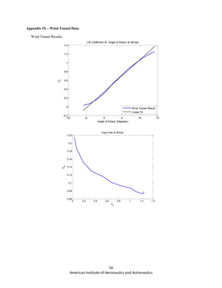
title('Lift Coefficient vs. Angle of Attack at 30mph')
xlabel('Angle of Attack (Degrees)')
ylabel('C_L')
figure
plot(CLs_cruise_30mph_corr_CG,CDs_cruise_30mph_corr_CG)
title('Drag Polar at 30mph')
xlabel('C_L')
ylabel('C_D')
figure
plot(CLs_cruise_30mph_corr_CG,CMs_cruise_30mph_corr_CG)
title('Moment Coefficient vs. Lift Coefficient at 30mph')
xlabel('C_L')
ylabel('C_m about CG')
figure
plot(alpha_cruise_30mph_corr,CLRs_cruise_30mph_corr_CG)
title('Rolling Moment Coefficient vs. Angle of Attack at 30mph')
xlabel('Angle of Attack (Degrees)')
ylabel('C_Lroll')
figure
plot(alpha_cruise_30mph_corr,CNs_cruise_30mph_corr_CG)
title('Yawing Moment Coefficient vs. Angle of Attack at 30mph')
xlabel('Angle of Attack (Degrees)')
ylabel('C_N')
%}
%% < < Speed = 60 mph > >
%import .dat file to matlab
[Data,SizeData] = importfile('cruise_60mph.dat', 2);
%Substract First Row which to substract Zero offset error
for i = 2:1:SizeData(1)
Data(i,:) = Data(i,:) - Data(1,:);
end
alpha_cruise_60mph = Data(2:end,1); %AoA vector in Deg.
Lift_cruise_60mph = Data(2:end,2); %Lift Vector in lbs.
Drag_cruise_60mph = Data(2:end,3); %Drag Vector in lbs.
Pitch_cruise_60mph = Data(2:end,4)*in_2_ft; %Pitching Moment
Vector in lbs*ft
Side_cruise_60mph = Data(2:end,5); %Sideforce Vector in lbs
Roll_cruise_60mph = Data(2:end,6)*in_2_ft; %Rolling Moment
Vector in lbs*ft
Yaw_cruise_60mph = Data(2:end,7)*in_2_ft; %Yawing Moment
Vector in lbs*ft
%First, we correct for no wind effect
Lift_cruise_60mph_corr = Lift_cruise_60mph - Lift_no_wind;
Drag_cruise_60mph_corr = Drag_cruise_60mph - Drag_no_wind;
Pitch_cruise_60mph_corr = Pitch_cruise_60mph - Pitch_no_wind;
Side_cruise_60mph_corr = Side_cruise_60mph - Side_no_wind;
Roll_cruise_60mph_corr = Roll_cruise_60mph - Roll_no_wind;
Yaw_cruise_60mph_corr = Yaw_cruise_60mph - Yaw_no_wind;
%Now, Since V is not 92 mph, we nondimensionalize Lift and
Drag
%To correct for no model in Lift and Drag to find other correction
factors
CLs_cruise_60mph_corr =
Lift_cruise_60mph_corr/(0.5*Density*(Vvec(end-1)^2)*Sw);
CDs_cruise_60mph_corr =
Drag_cruise_60mph_corr/(0.5*Density*(Vvec(end-1)^2)*Sw);
%Now we correct for no model error
CLs_cruise_60mph_corr = CLs_cruise_60mph_corr -
CLs_no_model;
CDs_cruise_60mph_corr = CDs_cruise_60mph_corr -
CDs_no_model;
%Now we compute CL squared to find K and CD0
CLs_cruise_60mph_CG_sq = CLs_cruise_60mph_corr.^2;](https://image.slidesharecdn.com/b6d5ca9f-0cd8-4fef-be65-ca3bfedf9c4c-151130202313-lva1-app6891/85/Paparrazzi_Final-1-46-320.jpg)
![46
American Institute of Aeronautics and Astronautics
%{
%We plot to have a sense of the results (Should be a straigth line)
figure
plot(CLs_cruise_60mph_CG_sq,CDs_cruise_60mph_corr)
%}
%We do a linear fit to compute the slope and the CD intercept
(CD0)
CL_sq_CD_60mph_Eq =
polyfit(CLs_cruise_60mph_CG_sq,CDs_cruise_60mph_corr,1);
%Compute K
K_cruise_60mph = CL_sq_CD_60mph_Eq(1);
%Compute e
e_osw_cruise_60mph = 1/(K_cruise_60mph*ARw*pi);
%Compute CD0
CD0_cruise_60mph = CL_sq_CD_60mph_Eq(2);
%Find Missing correction factors
Ewbt_cruise_60mph = (Sw/(4*Acs))*CD0_cruise_60mph;
Etot_cruise_60mph = Esbt + Ewbt_cruise_60mph +
Estrut_windshield;
%Compute Corrected dynamic pressure
q_corr_cruise_60mph = q_s(end-1)*(1+Etot_cruise_60mph)^2;
%Use Corrected dynamic pressure to compute all coefficients
CLs_cruise_60mph_corr =
Lift_cruise_60mph_corr/(q_corr_cruise_60mph*Sw);
CDs_cruise_60mph_corr =
Drag_cruise_60mph_corr/(q_corr_cruise_60mph*Sw);
CSFs_cruise_60mph_corr =
Side_cruise_60mph_corr/(q_corr_cruise_60mph*Sw);
CMs_cruise_60mph_corr =
Pitch_cruise_60mph_corr/(q_corr_cruise_60mph*Sw*cbar_w);
CLRs_cruise_60mph_corr =
Roll_cruise_60mph_corr/(q_corr_cruise_60mph*Sw*cbar_w);
CNs_cruise_60mph_corr =
Yaw_cruise_60mph_corr/(q_corr_cruise_60mph*Sw*cbar_w);
%Now we correct all coefficients for no model error
CLs_cruise_60mph_corr = CLs_cruise_60mph_corr -
CLs_no_model;
CDs_cruise_60mph_corr = CDs_cruise_60mph_corr -
CDs_no_model;
CSFs_cruise_60mph_corr = CSFs_cruise_60mph_corr -
CSFs_no_model;
CMs_cruise_60mph_corr = CMs_cruise_60mph_corr -
CMs_no_model;
CLRs_cruise_60mph_corr = CLRs_cruise_60mph_corr -
CLRs_no_model;
CNs_cruise_60mph_corr = CNs_cruise_60mph_corr -
CNs_no_model;
%Compute AoA correction Vector
Delta_alpha_cruise_60mph =
Delta*(1+Tau2)*(Sw/Acs)*(180/pi)*CLs_cruise_60mph_corr;
%Corrected AoA
alpha_cruise_60mph_corr = alpha_cruise_60mph +
Delta_alpha_cruise_60mph;
%Drag Wall Correction
Delta_Cd_cruise_60mph =
Delta*(Sw/Acs)*(CLs_cruise_60mph_corr.^2);
%Tail Moment Coefficient Correction Vector
Delta_Cm_CG_cruise_60mph =
DCmcg_Ddelta*(Sw/Acs)*(180/pi)*Delta*Tau2*...
CLs_cruise_60mph_corr;
%Now we translate the Loads and moments from Balance Center
to CG
%Loads_CG = Loads_Balance
%Moments_CG = Moment_Balance
CLs_cruise_60mph_corr_CG = CLs_cruise_60mph_corr;
CDs_cruise_60mph_corr_CG = CDs_cruise_60mph_corr +
Delta_Cd_cruise_60mph;
CSFs_cruise_60mph_corr_CG = CSFs_cruise_60mph_corr;
CMs_cruise_60mph_corr_CG = (CMs_cruise_60mph_corr +...
CLs_cruise_60mph_corr*(X_balance_CG/cbar_w)-...
CDs_cruise_60mph_corr*(Z_balance_CG/cbar_w)) -
Delta_Cm_CG_cruise_60mph;
CLRs_cruise_60mph_corr_CG = CLRs_cruise_60mph_corr -...
CSFs_cruise_60mph_corr*(Z_balance_CG/cbar_w);
CNs_cruise_60mph_corr_CG = CNs_cruise_60mph_corr +...
CSFs_cruise_60mph_corr*(X_balance_CG/cbar_w);
%{
%Plot Results for further Study
figure
plot(alpha_cruise_60mph_corr,CLs_cruise_60mph_corr_CG)
title('Lift Coefficient vs. Angle of Attack at 60mph')
xlabel('Angle of Attack (Degrees)')
ylabel('C_L')
figure
plot(CLs_cruise_60mph_corr_CG,CDs_cruise_60mph_corr_CG)
title('Drag Polar at 60mph')
xlabel('C_L')
ylabel('C_D')
figure
plot(CLs_cruise_60mph_corr_CG,CMs_cruise_60mph_corr_CG)
title('Moment Coefficient vs. Lift Coefficient at 60mph')
xlabel('C_L')
ylabel('C_m')
figure
plot(alpha_cruise_60mph_corr,CLRs_cruise_60mph_corr_CG)
title('Rolling Moment Coefficient vs. Angle of Attack at 60mph')
xlabel('Angle of Attack (Degrees)')
ylabel('C_Lroll')
figure
plot(alpha_cruise_60mph_corr,CNs_cruise_60mph_corr_CG)
title('Yawing Moment Coefficient vs. Angle of Attack at 60mph')
xlabel('Angle of Attack (Degrees)')
ylabel('C_N')
%}
%% < < Speed = 92 mph (Design Speed) > >
%import .dat file to matlab
[Data,SizeData] = importfile('cruise_92mph.dat', 2);
%Substract First Row which to substract Zero offset error
for i = 2:1:SizeData(1)
Data(i,:) = Data(i,:) - Data(1,:);
end
alpha_cruise_92mph = Data(2:end,1); %AoA vector in Deg.
Lift_cruise_92mph = Data(2:end,2); %Lift Vector in lbs.
Drag_cruise_92mph = Data(2:end,3); %Drag Vector in lbs.
Pitch_cruise_92mph = Data(2:end,4)*in_2_ft; %Pitching Moment
Vector in lbs*ft](https://image.slidesharecdn.com/b6d5ca9f-0cd8-4fef-be65-ca3bfedf9c4c-151130202313-lva1-app6891/85/Paparrazzi_Final-1-47-320.jpg)
![48
American Institute of Aeronautics and Astronautics
%{%}
%Plot Results for further Study
figure
plot(alpha_cruise_92mph_corr,CLs_cruise_92mph_corr_CG,'Line
Width',2)
hold on
plot(alpha_cruise_92mph_corr,CL_alpha_cruise_92mph_Eq,'--
k','Linewidth',2)
title('Lift Coefficient vs. Angle of Attack at 92mph')
xlabel('Angle of Attack (Degrees)')
ylabel('C_L')
legend('Wind Tunnel Result','Linear Fit','location','SouthEast')
figure
plot(CLs_cruise_92mph_corr_CG,CDs_cruise_92mph_corr_CG,'L
ineWidth',2)
title('Drag Polar at 92mph')
xlabel('C_L')
ylabel('C_D')
figure
plot(alpha_cruise_92mph_corr,CMs_cruise_92mph_corr_CG,'b','L
ineWidth',2)
hold on
plot(alpha_cruise_92mph_corr,CM_cruise_92mph_alpha_Eq,'--
k','LineWidth',2)
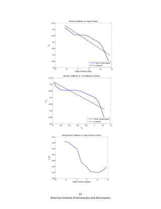
title('Moment Coefficient vs. Angle of Attack')
xlabel('Angle of Attack (Deg.)')
ylabel('C_m')
legend('Wind Tunnel Result','Linear Fit','Location','SouthEast')
figure
plot(CLs_cruise_92mph_corr_CG,CMs_cruise_92mph_corr_CG,'
b','LineWidth',2)
hold on
plot(CLs_cruise_92mph_corr_CG,CM_cruise_92mph_CL_Eq,'--
k','LineWidth',2)
title('Moment Coefficient vs. Lift Coefficient at 92mph')
xlabel('C_L')
ylabel('C_m')
legend('Wind Tunnel Result','LinearFit','location','SouthEast')
figure
plot(alpha_cruise_92mph_corr,CLRs_cruise_92mph_corr_CG,'Lin
eWidth',2)
title('Rolling Moment Coefficient vs. Angle of Attack at 92mph')
xlabel('Angle of Attack (Degrees)')
ylabel('C_Lroll')
figure
plot(alpha_cruise_92mph_corr,CNs_cruise_92mph_corr_CG,'Line
Width',2)
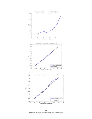
title('Yawing Moment Coefficient vs. Angle of Attack at 92mph')
xlabel('Angle of Attack (Degrees)')
ylabel('C_N')
%% Zero Reference for Stability Analysis
%import .dat file to matlab
[Data,SizeData] = importfile('zero_reference_control.dat', 2);
%Substract First Row which to substract Zero offset error
for i = 2:1:SizeData(1)
Data(i,:) = Data(i,:) - Data(1,:);
end
alpha_zero_reference_control = Data(2:end,1); %AoA vector in
Deg.
Lift_zero_reference_control = Data(2:end,2); %Lift Vector in lbs.
Drag_zero_reference_control = Data(2:end,3); %Drag Vector in
lbs.
Pitch_zero_reference_control = Data(2:end,4)*in_2_ft; %Pitching
Moment Vector in lbs*ft
Side_zero_reference_control = Data(2:end,5); %Sideforce Vector
in lbs
Roll_zero_reference_control = Data(2:end,6)*in_2_ft; %Rolling
Moment Vector in lbs*ft
Yaw_zero_reference_control = Data(2:end,7)*in_2_ft; %Yawing
Moment Vector in lbs*ft
%First, we correct for no wind effect
Lift_zero_reference_control_corr = Lift_zero_reference_control -
Lift_no_wind(4);
Drag_zero_reference_control_corr = Drag_zero_reference_control
- Drag_no_wind(4);
Pitch_zero_reference_control_corr = Pitch_zero_reference_control
- Pitch_no_wind(4);
Side_zero_reference_control_corr = Side_zero_reference_control -
Side_no_wind(4);
Roll_zero_reference_control_corr = Roll_zero_reference_control -
Roll_no_wind(4);
Yaw_zero_reference_control_corr = Yaw_zero_reference_control
- Yaw_no_wind(4);
%Use Corrected dynamic pressure to compute all coefficients
CLs_zero_reference_control_corr =
Lift_zero_reference_control_corr/(q_corr_cruise_30mph*Sw);
CDs_zero_reference_control_corr =
Drag_zero_reference_control_corr/(q_corr_cruise_30mph*Sw);
CSFs_zero_reference_control_corr =
Side_zero_reference_control_corr/(q_corr_cruise_30mph*Sw);
CMs_zero_reference_control_corr =
Pitch_zero_reference_control_corr/(q_corr_cruise_30mph*Sw*cba
r_w);
CLRs_zero_reference_control_corr =
Roll_zero_reference_control_corr/(q_corr_cruise_30mph*Sw*cbar
_w);
CNs_zero_reference_control_corr =
Yaw_zero_reference_control_corr/(q_corr_cruise_30mph*Sw*cba
r_w);
%Now we correct all coefficients for no model error
CLs_zero_reference_control_corr =
CLs_zero_reference_control_corr - CLs_no_model;
CDs_zero_reference_control_corr =
CDs_zero_reference_control_corr - CDs_no_model;
CSFs_zero_reference_control_corr =
CSFs_zero_reference_control_corr - CSFs_no_model;
CMs_zero_reference_control_corr =
CMs_zero_reference_control_corr - CMs_no_model;
CLRs_zero_reference_control_corr =
CLRs_zero_reference_control_corr - CLRs_no_model;
CNs_zero_reference_control_corr =
CNs_zero_reference_control_corr - CNs_no_model;
%Compute AoA correction Vector
Delta_alpha_zero_reference_control =
Delta*(1+Tau2)*(Sw/Acs)*(180/pi)*CLs_zero_reference_control_
corr;
%Corrected AoA
alpha_zero_reference_control_corr =
alpha_zero_reference_control +
Delta_alpha_zero_reference_control;
%Drag Wall Correction
Delta_Cd_zero_reference_control =
Delta*(Sw/Acs)*(CLs_zero_reference_control_corr.^2);](https://image.slidesharecdn.com/b6d5ca9f-0cd8-4fef-be65-ca3bfedf9c4c-151130202313-lva1-app6891/85/Paparrazzi_Final-1-49-320.jpg)
![49
American Institute of Aeronautics and Astronautics
%Tail Moment Coefficient Correction Vector
Delta_Cm_CG_zero_reference_control =
DCmcg_Ddelta*(Sw/Acs)*(180/pi)*Delta*Tau2*...
CLs_zero_reference_control_corr;
%Now we translate the Loads and moments from Balance Center
to CG
%Loads_CG = Loads_Balance
%Moments_CG = Moment_Balance
CLs_zero_reference_control_corr_CG =
CLs_zero_reference_control_corr;
CDs_zero_reference_control_corr_CG =
CDs_zero_reference_control_corr +
Delta_Cd_zero_reference_control;
CSFs_zero_reference_control_corr_CG =
CSFs_zero_reference_control_corr;
CMs_zero_reference_control_corr_CG =
(CMs_zero_reference_control_corr +...
CLs_zero_reference_control_corr*(X_balance_CG/cbar_w)-...
CDs_zero_reference_control_corr*(Z_balance_CG/cbar_w)) -
Delta_Cm_CG_zero_reference_control;
CLRs_zero_reference_control_corr_CG =
CLRs_zero_reference_control_corr -...
CSFs_zero_reference_control_corr*(Z_balance_CG/cbar_w);
CNs_zero_reference_control_corr_CG =
CNs_zero_reference_control_corr +...
CSFs_zero_reference_control_corr*(X_balance_CG/cbar_w);
%% Roll Body Stability Analysis
%% < < Left Wing 11 Degrees Down > >
%Import .dat File into Matlab
[Data,SizeData] = importfile('roll_left_wing_11deg_down.dat', 2);
%Substract First Row which to substract Zero offset error
for i = 2:1:SizeData(1)
Data(i,:) = Data(i,:) - Data(1,:);
end
alpha_roll_11deg_down = Data(2:end,1); %AoA vector in Deg.
Lift_roll_11deg_down = Data(2:end,2); %Lift Vector in lbs.
Drag_roll_11deg_down = Data(2:end,3); %Drag Vector in lbs.
Pitch_roll_11deg_down = Data(2:end,4)*in_2_ft; %Pitching
Moment Vector in lbs*ft
Side_roll_11deg_down = Data(2:end,5); %Sideforce Vector in lbs
Roll_roll_11deg_down = Data(2:end,6)*in_2_ft; %Rolling
Moment Vector in lbs*ft
Yaw_roll_11deg_down = Data(2:end,7)*in_2_ft; %Yawing
Moment Vector in lbs*ft
%First, we correct for no wind effect
Lift_roll_11deg_down_corr = Lift_roll_11deg_down -
Lift_no_wind(4);
Drag_roll_11deg_down_corr = Drag_roll_11deg_down -
Drag_no_wind(4);
Pitch_roll_11deg_down_corr = Pitch_roll_11deg_down -
Pitch_no_wind(4);
Side_roll_11deg_down_corr = Side_roll_11deg_down -
Side_no_wind(4);
Roll_roll_11deg_down_corr = Roll_roll_11deg_down -
Roll_no_wind(4);
Yaw_roll_11deg_down_corr = Yaw_roll_11deg_down -
Yaw_no_wind(4);
%Use Corrected dynamic pressure to compute all coefficients
CLs_roll_11deg_down_corr =
Lift_roll_11deg_down_corr/(q_corr_cruise_30mph*Sw);
CDs_roll_11deg_down_corr =
Drag_roll_11deg_down_corr/(q_corr_cruise_30mph*Sw);
CSFs_roll_11deg_down_corr =
Side_roll_11deg_down_corr/(q_corr_cruise_30mph*Sw);
CMs_roll_11deg_down_corr =
Pitch_roll_11deg_down_corr/(q_corr_cruise_30mph*Sw*cbar_w);
CLRs_roll_11deg_down_corr =
Roll_roll_11deg_down_corr/(q_corr_cruise_30mph*Sw*cbar_w);
CNs_roll_11deg_down_corr =
Yaw_roll_11deg_down_corr/(q_corr_cruise_30mph*Sw*cbar_w);
%Now we correct all coefficients for no model error
CLs_roll_11deg_down_corr = CLs_roll_11deg_down_corr -
CLs_no_model;
CDs_roll_11deg_down_corr = CDs_roll_11deg_down_corr -
CDs_no_model;
CSFs_roll_11deg_down_corr = CSFs_roll_11deg_down_corr -
CSFs_no_model;
CMs_roll_11deg_down_corr = CMs_roll_11deg_down_corr -
CMs_no_model;
CLRs_roll_11deg_down_corr = CLRs_roll_11deg_down_corr -
CLRs_no_model;
CNs_roll_11deg_down_corr = CNs_roll_11deg_down_corr -
CNs_no_model;
%Compute AoA correction Vector
Delta_alpha_roll_11deg_down =
Delta*(1+Tau2)*(Sw/Acs)*(180/pi)*CLs_roll_11deg_down_corr;
%Corrected AoA
alpha_roll_11deg_down_corr = alpha_roll_11deg_down +
Delta_alpha_roll_11deg_down;
%Drag Wall Correction
Delta_Cd_roll_11deg_down =
Delta*(Sw/Acs)*(CLs_roll_11deg_down_corr.^2);
%Tail Moment Coefficient Correction Vector
Delta_Cm_CG_roll_11deg_down =
DCmcg_Ddelta*(Sw/Acs)*(180/pi)*Delta*Tau2*...
CLs_roll_11deg_down_corr;
%Now we translate the Loads and moments from Balance Center
to CG
%Loads_CG = Loads_Balance
%Moments_CG = Moment_Balance
CLs_roll_11deg_down_corr_CG = CLs_roll_11deg_down_corr;
CDs_roll_11deg_down_corr_CG = CDs_roll_11deg_down_corr +
Delta_Cd_roll_11deg_down;
CSFs_roll_11deg_down_corr_CG = CSFs_roll_11deg_down_corr;
CMs_roll_11deg_down_corr_CG = (CMs_roll_11deg_down_corr
+...
CLs_roll_11deg_down_corr*(X_balance_CG/cbar_w)-...
CDs_roll_11deg_down_corr*(Z_balance_CG/cbar_w)) -
Delta_Cm_CG_roll_11deg_down;
CLRs_roll_11deg_down_corr_CG = CLRs_roll_11deg_down_corr
-...
CSFs_roll_11deg_down_corr*(Z_balance_CG/cbar_w);
CNs_roll_11deg_down_corr_CG = CNs_roll_11deg_down_corr
+...
CSFs_roll_11deg_down_corr*(X_balance_CG/cbar_w);
%% < < Left Wing 8 Degrees Up > >
%Import .dat File into Matlab
[Data,SizeData] = importfile('roll_left_wing_8deg_up.dat', 2);](https://image.slidesharecdn.com/b6d5ca9f-0cd8-4fef-be65-ca3bfedf9c4c-151130202313-lva1-app6891/85/Paparrazzi_Final-1-50-320.jpg)
![50
American Institute of Aeronautics and Astronautics
%Substract First Row which to substract Zero offset error
for i = 2:1:SizeData(1)
Data(i,:) = Data(i,:) - Data(1,:);
end
alpha_roll_8deg_up = Data(2:end,1); %AoA vector in Deg.
Lift_roll_8deg_up = Data(2:end,2); %Lift Vector in lbs.
Drag_roll_8deg_up = Data(2:end,3); %Drag Vector in lbs.
Pitch_roll_8deg_up = Data(2:end,4)*in_2_ft; %Pitching Moment
Vector in lbs*ft
Side_roll_8deg_up = Data(2:end,5); %Sideforce Vector in lbs
Roll_roll_8deg_up = Data(2:end,6)*in_2_ft; %Rolling Moment
Vector in lbs*ft
Yaw_roll_8deg_up = Data(2:end,7)*in_2_ft; %Yawing Moment
Vector in lbs*ft
%First, we correct for no wind effect
Lift_roll_8deg_up_corr = Lift_roll_8deg_up - Lift_no_wind(4);
Drag_roll_8deg_up_corr = Drag_roll_8deg_up -
Drag_no_wind(4);
Pitch_roll_8deg_up_corr = Pitch_roll_8deg_up -
Pitch_no_wind(4);
Side_roll_8deg_up_corr = Side_roll_8deg_up - Side_no_wind(4);
Roll_roll_8deg_up_corr = Roll_roll_8deg_up - Roll_no_wind(4);
Yaw_roll_8deg_up_corr = Yaw_roll_8deg_up - Yaw_no_wind(4);
%Use Corrected dynamic pressure to compute all coefficients
CLs_roll_8deg_up_corr =
Lift_roll_8deg_up_corr/(q_corr_cruise_30mph*Sw);
CDs_roll_8deg_up_corr =
Drag_roll_8deg_up_corr/(q_corr_cruise_30mph*Sw);
CSFs_roll_8deg_up_corr =
Side_roll_8deg_up_corr/(q_corr_cruise_30mph*Sw);
CMs_roll_8deg_up_corr =
Pitch_roll_8deg_up_corr/(q_corr_cruise_30mph*Sw*cbar_w);
CLRs_roll_8deg_up_corr =
Roll_roll_8deg_up_corr/(q_corr_cruise_30mph*Sw*cbar_w);
CNs_roll_8deg_up_corr =
Yaw_roll_8deg_up_corr/(q_corr_cruise_30mph*Sw*cbar_w);
%Now we correct all coefficients for no model error
CLs_roll_8deg_up_corr = CLs_roll_8deg_up_corr -
CLs_no_model;
CDs_roll_8deg_up_corr = CDs_roll_8deg_up_corr -
CDs_no_model;
CSFs_roll_8deg_up_corr = CSFs_roll_8deg_up_corr -
CSFs_no_model;
CMs_roll_8deg_up_corr = CMs_roll_8deg_up_corr -
CMs_no_model;
CLRs_roll_8deg_up_corr = CLRs_roll_8deg_up_corr -
CLRs_no_model;
CNs_roll_8deg_up_corr = CNs_roll_8deg_up_corr -
CNs_no_model;
%Compute AoA correction Vector
Delta_alpha_roll_8deg_up =
Delta*(1+Tau2)*(Sw/Acs)*(180/pi)*CLs_roll_8deg_up_corr;
%Corrected AoA
alpha_roll_8deg_up_corr = alpha_roll_8deg_up +
Delta_alpha_roll_8deg_up;
%Drag Wall Correction
Delta_Cd_roll_8deg_up =
Delta*(Sw/Acs)*(CLs_roll_8deg_up_corr.^2);
%Tail Moment Coefficient Correction Vector
Delta_Cm_CG_roll_8deg_up =
DCmcg_Ddelta*(Sw/Acs)*(180/pi)*Delta*Tau2*...
CLs_roll_8deg_up_corr;
%Now we translate the Loads and moments from Balance Center
to CG
%Loads_CG = Loads_Balance
%Moments_CG = Moment_Balance
CLs_roll_8deg_up_corr_CG = CLs_roll_8deg_up_corr;
CDs_roll_8deg_up_corr_CG = CDs_roll_8deg_up_corr +
Delta_Cd_roll_8deg_up;
CSFs_roll_8deg_up_corr_CG = CSFs_roll_8deg_up_corr;
CMs_roll_8deg_up_corr_CG = (CMs_roll_8deg_up_corr +...
CLs_roll_8deg_up_corr*(X_balance_CG/cbar_w)-...
CDs_roll_8deg_up_corr*(Z_balance_CG/cbar_w)) -
Delta_Cm_CG_roll_8deg_up;
CLRs_roll_8deg_up_corr_CG = CLRs_roll_8deg_up_corr -...
CSFs_roll_8deg_up_corr*(Z_balance_CG/cbar_w);
CNs_roll_8deg_up_corr_CG = CNs_roll_8deg_up_corr +...
CSFs_roll_8deg_up_corr*(X_balance_CG/cbar_w);
%% < < Left Wing 16 Degrees Up > >
%Import .dat File into Matlab
[Data,SizeData] = importfile('roll_left_wing_16deg_up.dat', 2);
%Substract First Row which to substract Zero offset error
for i = 2:1:SizeData(1)
Data(i,:) = Data(i,:) - Data(1,:);
end
alpha_roll_16deg_up = Data(2:end,1); %AoA vector in Deg.
Lift_roll_16deg_up = Data(2:end,2); %Lift Vector in lbs.
Drag_roll_16deg_up = Data(2:end,3); %Drag Vector in lbs.
Pitch_roll_16deg_up = Data(2:end,4)*in_2_ft; %Pitching Moment
Vector in lbs*ft
Side_roll_16deg_up = Data(2:end,5); %Sideforce Vector in lbs
Roll_roll_16deg_up = Data(2:end,6)*in_2_ft; %Rolling Moment
Vector in lbs*ft
Yaw_roll_16deg_up = Data(2:end,7)*in_2_ft; %Yawing Moment
Vector in lbs*ft
%First, we correct for no wind effect
Lift_roll_16deg_up_corr = Lift_roll_16deg_up - Lift_no_wind(4);
Drag_roll_16deg_up_corr = Drag_roll_16deg_up -
Drag_no_wind(4);
Pitch_roll_16deg_up_corr = Pitch_roll_16deg_up -
Pitch_no_wind(4);
Side_roll_16deg_up_corr = Side_roll_16deg_up -
Side_no_wind(4);
Roll_roll_16deg_up_corr = Roll_roll_16deg_up -
Roll_no_wind(4);
Yaw_roll_16deg_up_corr = Yaw_roll_16deg_up -
Yaw_no_wind(4);
%Use Corrected dynamic pressure to compute all coefficients
CLs_roll_16deg_up_corr =
Lift_roll_16deg_up_corr/(q_corr_cruise_30mph*Sw);
CDs_roll_16deg_up_corr =
Drag_roll_16deg_up_corr/(q_corr_cruise_30mph*Sw);
CSFs_roll_16deg_up_corr =
Side_roll_16deg_up_corr/(q_corr_cruise_30mph*Sw);
CMs_roll_16deg_up_corr =
Pitch_roll_16deg_up_corr/(q_corr_cruise_30mph*Sw*cbar_w);
CLRs_roll_16deg_up_corr =
Roll_roll_16deg_up_corr/(q_corr_cruise_30mph*Sw*cbar_w);
CNs_roll_16deg_up_corr =
Yaw_roll_16deg_up_corr/(q_corr_cruise_30mph*Sw*cbar_w);
%Now we correct all coefficients for no model error](https://image.slidesharecdn.com/b6d5ca9f-0cd8-4fef-be65-ca3bfedf9c4c-151130202313-lva1-app6891/85/Paparrazzi_Final-1-51-320.jpg)
![51
American Institute of Aeronautics and Astronautics
CLs_roll_16deg_up_corr = CLs_roll_16deg_up_corr -
CLs_no_model;
CDs_roll_16deg_up_corr = CDs_roll_16deg_up_corr -
CDs_no_model;
CSFs_roll_16deg_up_corr = CSFs_roll_16deg_up_corr -
CSFs_no_model;
CMs_roll_16deg_up_corr = CMs_roll_16deg_up_corr -
CMs_no_model;
CLRs_roll_16deg_up_corr = CLRs_roll_16deg_up_corr -
CLRs_no_model;
CNs_roll_16deg_up_corr = CNs_roll_16deg_up_corr -
CNs_no_model;
%Compute AoA correction Vector
Delta_alpha_roll_16deg_up =
Delta*(1+Tau2)*(Sw/Acs)*(180/pi)*CLs_roll_16deg_up_corr;
%Corrected AoA
alpha_roll_16deg_up_corr = alpha_roll_16deg_up +
Delta_alpha_roll_16deg_up;
%Drag Wall Correction
Delta_Cd_roll_16deg_up =
Delta*(Sw/Acs)*(CLs_roll_16deg_up_corr.^2);
%Tail Moment Coefficient Correction Vector
Delta_Cm_CG_roll_16deg_up =
DCmcg_Ddelta*(Sw/Acs)*(180/pi)*Delta*Tau2*...
CLs_roll_16deg_up_corr;
%Now we translate the Loads and moments from Balance Center
to CG
%Loads_CG = Loads_Balance
%Moments_CG = Moment_Balance
CLs_roll_16deg_up_corr_CG = CLs_roll_16deg_up_corr;
CDs_roll_16deg_up_corr_CG = CDs_roll_16deg_up_corr +
Delta_Cd_roll_16deg_up;
CSFs_roll_16deg_up_corr_CG = CSFs_roll_16deg_up_corr;
CMs_roll_16deg_up_corr_CG = (CMs_roll_16deg_up_corr +...
CLs_roll_16deg_up_corr*(X_balance_CG/cbar_w)-...
CDs_roll_16deg_up_corr*(Z_balance_CG/cbar_w)) -
Delta_Cm_CG_roll_16deg_up;
CLRs_roll_16deg_up_corr_CG = CLRs_roll_16deg_up_corr -...
CSFs_roll_16deg_up_corr*(Z_balance_CG/cbar_w);
CNs_roll_16deg_up_corr_CG = CNs_roll_16deg_up_corr +...
CSFs_roll_16deg_up_corr*(X_balance_CG/cbar_w);
CLRs_wing_incidence = [CLRs_roll_11deg_down_corr_CG...
CLRs_zero_reference_control_corr_CG...
CLRs_roll_8deg_up_corr_CG...
CLRs_roll_16deg_up_corr_CG];
CNs_wing_incidence = [CNs_roll_11deg_down_corr_CG...
CNs_zero_reference_control_corr_CG...
CNs_roll_8deg_up_corr_CG...
CNs_roll_16deg_up_corr_CG];
Wing_incidence_angles = [-11 0 8 16];
CLR_Wing_incidence_fit =
polyfit(Wing_incidence_angles,CLRs_wing_incidence,1);
CN_Wing_incidecne_fit =
polyfit(Wing_incidence_angles,CNs_wing_incidence,1);
CLRs_Equation_incidence =
polyval(CLR_Wing_incidence_fit,Wing_incidence_angles);
CNs_Equation_incidence =
polyval(CN_Wing_incidecne_fit,Wing_incidence_angles);
%Compute Stability Derivative
DCLroll_Di = CLR_Wing_incidence_fit(1); %1/deg
DCN_Di = CN_Wing_incidecne_fit(1); %SHould be negative, it is
positive probably due to decrease in Drag as AoA increases!!
%{%}
figure
plot(Wing_incidence_angles,CLRs_wing_incidence,'b','LineWidth'
,2)
hold on
plot(Wing_incidence_angles,CLRs_Equation_incidence,'--
k','LineWidth',2)
title('Rolling Moment Coefficient vs. Wing Incidence Angle')
xlabel('Wing Incidence Angle (Deg.)')
ylabel('C_Lroll')
legend('Wind Tunel Result','Linear Fit','Location','SouthEast')
figure
plot(Wing_incidence_angles,CNs_wing_incidence,'b','LineWidth',
2)
hold on
plot(Wing_incidence_angles,CNs_Equation_incidence,'--
k','LineWidth',2)
title('Yawing Moment Coefficient vs. Wing Incidence Angle')
xlabel('Wing Incidence Angle (Deg.)')
ylabel('C_N')
legend('Wind Tunel Result','Linear Fit','Location','SouthEast')
%% Yaw Body Stability Analysis
% < < Sideslip = 8 Deg. Counterclockwise > >
%Import .dat File into Matlab
[Data,SizeData] = importfile('yaw_8deg_counterclockwise.dat', 2);
%Substract First Row which to substract Zero offset error
for i = 2:1:SizeData(1)
Data(i,:) = Data(i,:) - Data(1,:);
end
alpha_yaw_8deg_counter = Data(2:end,1); %AoA vector in Deg.
Lift_yaw_8deg_counter = Data(2:end,2); %Lift Vector in lbs.
Drag_yaw_8deg_counter = Data(2:end,3); %Drag Vector in lbs.
Pitch_yaw_8deg_counter = Data(2:end,4)*in_2_ft; %Pitching
Moment Vector in lbs*ft
Side_yaw_8deg_counter = Data(2:end,5); %Sideforce Vector in
lbs
Roll_yaw_8deg_counter = Data(2:end,6)*in_2_ft; %Rolling
Moment Vector in lbs*ft
Yaw_yaw_8deg_counter = Data(2:end,7)*in_2_ft; %Yawing
Moment Vector in lbs*ft
%First, we correct for no wind effect
Lift_yaw_8deg_counter_corr = Lift_yaw_8deg_counter -
Lift_no_wind(4);
Drag_yaw_8deg_counter_corr = Drag_yaw_8deg_counter -
Drag_no_wind(4);
Pitch_yaw_8deg_counter_corr = Pitch_yaw_8deg_counter -
Pitch_no_wind(4);
Side_yaw_8deg_counter_corr = Side_yaw_8deg_counter -
Side_no_wind(4);
Roll_yaw_8deg_counter_corr = Roll_yaw_8deg_counter -
Roll_no_wind(4);
Yaw_yaw_8deg_counter_corr = Yaw_yaw_8deg_counter -
Yaw_no_wind(4);
%Use Corrected dynamic pressure to compute all coefficients
CLs_yaw_8deg_counter_corr =
Lift_yaw_8deg_counter_corr/(q_corr_cruise_30mph*Sw);](https://image.slidesharecdn.com/b6d5ca9f-0cd8-4fef-be65-ca3bfedf9c4c-151130202313-lva1-app6891/85/Paparrazzi_Final-1-52-320.jpg)
![52
American Institute of Aeronautics and Astronautics
CDs_yaw_8deg_counter_corr =
Drag_yaw_8deg_counter_corr/(q_corr_cruise_30mph*Sw);
CSFs_yaw_8deg_counter_corr =
Side_yaw_8deg_counter_corr/(q_corr_cruise_30mph*Sw);
CMs_yaw_8deg_counter_corr =
Pitch_yaw_8deg_counter_corr/(q_corr_cruise_30mph*Sw*cbar_w
);
CLRs_yaw_8deg_counter_corr =
Roll_yaw_8deg_counter_corr/(q_corr_cruise_30mph*Sw*cbar_w)
;
CNs_yaw_8deg_counter_corr =
Yaw_yaw_8deg_counter_corr/(q_corr_cruise_30mph*Sw*cbar_w
);
%Now we correct all coefficients for no model error
CLs_yaw_8deg_counter_corr = CLs_yaw_8deg_counter_corr -
CLs_no_model;
CDs_yaw_8deg_counter_corr = CDs_yaw_8deg_counter_corr -
CDs_no_model;
CSFs_yaw_8deg_counter_corr = CSFs_yaw_8deg_counter_corr -
CSFs_no_model;
CMs_yaw_8deg_counter_corr = CMs_yaw_8deg_counter_corr -
CMs_no_model;
CLRs_yaw_8deg_counter_corr = CLRs_yaw_8deg_counter_corr -
CLRs_no_model;
CNs_yaw_8deg_counter_corr = CNs_yaw_8deg_counter_corr -
CNs_no_model;
%Compute AoA correction Vector
Delta_alpha_yaw_8deg_counter =
Delta*(1+Tau2)*(Sw/Acs)*(180/pi)*CLs_yaw_8deg_counter_corr
;
%Corrected AoA
alpha_yaw_8deg_counter_corr = alpha_yaw_8deg_counter +
Delta_alpha_yaw_8deg_counter;
%Drag Wall Correction
Delta_Cd_yaw_8deg_counter =
Delta*(Sw/Acs)*(CLs_yaw_8deg_counter_corr.^2);
%Tail Moment Coefficient Correction Vector
Delta_Cm_CG_yaw_8deg_counter =
DCmcg_Ddelta*(Sw/Acs)*(180/pi)*Delta*Tau2*...
CLs_yaw_8deg_counter_corr;
%Now we translate the Loads and moments from Balance Center
to CG
%Loads_CG = Loads_Balance
%Moments_CG = Moment_Balance
CLs_yaw_8deg_counter_corr_CG =
CLs_yaw_8deg_counter_corr;
CDs_yaw_8deg_counter_corr_CG = CDs_yaw_8deg_counter_corr
+ Delta_Cd_yaw_8deg_counter;
CSFs_yaw_8deg_counter_corr_CG =
CSFs_yaw_8deg_counter_corr;
CMs_yaw_8deg_counter_corr_CG =
(CMs_yaw_8deg_counter_corr +...
CLs_yaw_8deg_counter_corr*(X_balance_CG/cbar_w)-...
CDs_yaw_8deg_counter_corr*(Z_balance_CG/cbar_w)) -
Delta_Cm_CG_yaw_8deg_counter;
CLRs_yaw_8deg_counter_corr_CG =
CLRs_yaw_8deg_counter_corr -...
CSFs_yaw_8deg_counter_corr*(Z_balance_CG/cbar_w);
CNs_yaw_8deg_counter_corr_CG = CNs_yaw_8deg_counter_corr
+...
CSFs_yaw_8deg_counter_corr*(X_balance_CG/cbar_w);
% < < Sideslip = 9 Deg. clockwise > >
%Import .dat File into Matlab
[Data,SizeData] = importfile('yaw_9deg_clockwise.dat', 2);
%Substract First Row which to substract Zero offset error
for i = 2:1:SizeData(1)
Data(i,:) = Data(i,:) - Data(1,:);
end
alpha_yaw_9deg_colockw = Data(2:end,1); %AoA vector in Deg.
Lift_yaw_9deg_colockw = Data(2:end,2); %Lift Vector in lbs.
Drag_yaw_9deg_colockw = Data(2:end,3); %Drag Vector in lbs.
Pitch_yaw_9deg_colockw = Data(2:end,4)*in_2_ft; %Pitching
Moment Vector in lbs*ft
Side_yaw_9deg_colockw = Data(2:end,5); %Sideforce Vector in
lbs
Roll_yaw_9deg_colockw = Data(2:end,6)*in_2_ft; %Rolling
Moment Vector in lbs*ft
Yaw_yaw_9deg_colockw = Data(2:end,7)*in_2_ft; %Yawing
Moment Vector in lbs*ft
%First, we correct for no wind effect
Lift_yaw_9deg_colockw_corr = Lift_yaw_9deg_colockw -
Lift_no_wind(4);
Drag_yaw_9deg_colockw_corr = Drag_yaw_9deg_colockw -
Drag_no_wind(4);
Pitch_yaw_9deg_colockw_corr = Pitch_yaw_9deg_colockw -
Pitch_no_wind(4);
Side_yaw_9deg_colockw_corr = Side_yaw_9deg_colockw -
Side_no_wind(4);
Roll_yaw_9deg_colockw_corr = Roll_yaw_9deg_colockw -
Roll_no_wind(4);
Yaw_yaw_9deg_colockw_corr = Yaw_yaw_9deg_colockw -
Yaw_no_wind(4);
%Use Corrected dynamic pressure to compute all coefficients
CLs_yaw_9deg_colockw_corr =
Lift_yaw_9deg_colockw_corr/(q_corr_cruise_30mph*Sw);
CDs_yaw_9deg_colockw_corr =
Drag_yaw_9deg_colockw_corr/(q_corr_cruise_30mph*Sw);
CSFs_yaw_9deg_colockw_corr =
Side_yaw_9deg_colockw_corr/(q_corr_cruise_30mph*Sw);
CMs_yaw_9deg_colockw_corr =
Pitch_yaw_9deg_colockw_corr/(q_corr_cruise_30mph*Sw*cbar_
w);
CLRs_yaw_9deg_colockw_corr =
Roll_yaw_9deg_colockw_corr/(q_corr_cruise_30mph*Sw*cbar_w
);
CNs_yaw_9deg_colockw_corr =
Yaw_yaw_9deg_colockw_corr/(q_corr_cruise_30mph*Sw*cbar_
w);
%Now we correct all coefficients for no model error
CLs_yaw_9deg_colockw_corr = CLs_yaw_9deg_colockw_corr -
CLs_no_model;
CDs_yaw_9deg_colockw_corr = CDs_yaw_9deg_colockw_corr -
CDs_no_model;
CSFs_yaw_9deg_colockw_corr = CSFs_yaw_9deg_colockw_corr
- CSFs_no_model;
CMs_yaw_9deg_colockw_corr = CMs_yaw_9deg_colockw_corr -
CMs_no_model;
CLRs_yaw_9deg_colockw_corr = CLRs_yaw_9deg_colockw_corr
- CLRs_no_model;
CNs_yaw_9deg_colockw_corr = CNs_yaw_9deg_colockw_corr -
CNs_no_model;
%Compute AoA correction Vector](https://image.slidesharecdn.com/b6d5ca9f-0cd8-4fef-be65-ca3bfedf9c4c-151130202313-lva1-app6891/85/Paparrazzi_Final-1-53-320.jpg)
![53
American Institute of Aeronautics and Astronautics
Delta_alpha_yaw_9deg_colockw =
Delta*(1+Tau2)*(Sw/Acs)*(180/pi)*CLs_yaw_9deg_colockw_cor
r;
%Corrected AoA
alpha_yaw_9deg_colockw_corr = alpha_yaw_9deg_colockw +
Delta_alpha_yaw_9deg_colockw;
%Drag Wall Correction
Delta_Cd_yaw_9deg_colockw =
Delta*(Sw/Acs)*(CLs_yaw_9deg_colockw_corr.^2);
%Tail Moment Coefficient Correction Vector
Delta_Cm_CG_yaw_9deg_colockw =
DCmcg_Ddelta*(Sw/Acs)*(180/pi)*Delta*Tau2*...
CLs_yaw_9deg_colockw_corr;
%Now we translate the Loads and moments from Balance Center
to CG
%Loads_CG = Loads_Balance
%Moments_CG = Moment_Balance
CLs_yaw_9deg_colockw_corr_CG =
CLs_yaw_9deg_colockw_corr;
CDs_yaw_9deg_colockw_corr_CG =
CDs_yaw_9deg_colockw_corr + Delta_Cd_yaw_9deg_colockw;
CSFs_yaw_9deg_colockw_corr_CG =
CSFs_yaw_9deg_colockw_corr;
CMs_yaw_9deg_colockw_corr_CG =
(CMs_yaw_9deg_colockw_corr +...
CLs_yaw_9deg_colockw_corr*(X_balance_CG/cbar_w)-...
CDs_yaw_9deg_colockw_corr*(Z_balance_CG/cbar_w)) -
Delta_Cm_CG_yaw_9deg_colockw;
CLRs_yaw_9deg_colockw_corr_CG =
CLRs_yaw_9deg_colockw_corr -...
CSFs_yaw_9deg_colockw_corr*(Z_balance_CG/cbar_w);
CNs_yaw_9deg_colockw_corr_CG =
CNs_yaw_9deg_colockw_corr +...
CSFs_yaw_9deg_colockw_corr*(X_balance_CG/cbar_w);
CNs_beta_sweep = [CNs_yaw_8deg_counter_corr_CG...
CNs_zero_reference_control_corr_CG...
CNs_yaw_9deg_colockw_corr_CG];
CLRs_beta_sweep = [CLRs_yaw_8deg_counter_corr_CG...
CLRs_zero_reference_control_corr_CG...
CLRs_yaw_9deg_colockw_corr_CG];
beta_angles = [-8 0 9];
CN_beta_fit = polyfit(beta_angles,CNs_beta_sweep,1);
CLR_beta_fit = polyfit(beta_angles,CLRs_beta_sweep,1);
CLRs_Equation_beta = polyval(CLR_beta_fit,beta_angles);
CNs_Equation_beta = polyval(CN_beta_fit,beta_angles);
%Compute Stability Derivative
DCLroll_DBeta = CLR_beta_fit(1); %1/deg
DCN_DBeta = CN_beta_fit(1);
%{%}
figure
plot(beta_angles,CLRs_beta_sweep,'b','LineWidth',2)
hold on
plot(beta_angles,CLRs_Equation_beta,'--k','LineWidth',2)
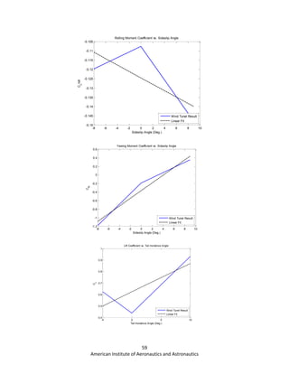
title('Rolling Moment Coefficient vs. Sideslip Angle')
xlabel('Sideslip Angle (Deg.)')
ylabel('C_Lroll')
legend('Wind Tunel Result','Linear Fit','Location','SouthEast')
figure
plot(beta_angles,CNs_beta_sweep,'b','LineWidth',2)
hold on
plot(beta_angles,CNs_Equation_beta,'--k','LineWidth',2)
title('Yawing Moment Coefficient vs. Sideslip Angle')
xlabel('Sideslip Angle (Deg.)')
ylabel('C_N')
legend('Wind Tunel Result','Linear Fit','Location','SouthEast')
%% Pitch Body Stability Analysis
%% < < Tail 5 Degrees Down > >
%Import .dat File into Matlab
[Data,SizeData] = importfile('pitch_5deg_down.dat', 2);
%Substract First Row which to substract Zero offset error
for i = 2:1:SizeData(1)
Data(i,:) = Data(i,:) - Data(1,:);
end
alpha_pitch_5deg_down = Data(2:end,1); %AoA vector in Deg.
Lift_pitch_5deg_down = Data(2:end,2); %Lift Vector in lbs.
Drag_pitch_5deg_down = Data(2:end,3); %Drag Vector in lbs.
Pitch_pitch_5deg_down = Data(2:end,4)*in_2_ft; %Pitching
Moment Vector in lbs*ft
Side_pitch_5deg_down = Data(2:end,5); %Sideforce Vector in lbs
Roll_pitch_5deg_down = Data(2:end,6)*in_2_ft; %Rolling
Moment Vector in lbs*ft
Yaw_pitch_5deg_down = Data(2:end,7)*in_2_ft; %Yawing
Moment Vector in lbs*ft
%First, we correct for no wind effect
Lift_pitch_5deg_down_corr = Lift_pitch_5deg_down -
Lift_no_wind(4);
Drag_pitch_5deg_down_corr = Drag_pitch_5deg_down -
Drag_no_wind(4);
Pitch_pitch_5deg_down_corr = Pitch_pitch_5deg_down -
Pitch_no_wind(4);
Side_pitch_5deg_down_corr = Side_pitch_5deg_down -
Side_no_wind(4);
Roll_pitch_5deg_down_corr = Roll_pitch_5deg_down -
Roll_no_wind(4);
Yaw_pitch_5deg_down_corr = Yaw_pitch_5deg_down -
Yaw_no_wind(4);
%Use Corrected dynamic pressure to compute all coefficients
CLs_pitch_5deg_down_corr =
Lift_pitch_5deg_down_corr/(q_corr_cruise_30mph*Sw);
CDs_pitch_5deg_down_corr =
Drag_pitch_5deg_down_corr/(q_corr_cruise_30mph*Sw);
CSFs_pitch_5deg_down_corr =
Side_pitch_5deg_down_corr/(q_corr_cruise_30mph*Sw);
CMs_pitch_5deg_down_corr =
Pitch_pitch_5deg_down_corr/(q_corr_cruise_30mph*Sw*cbar_w)
;
CLRs_pitch_5deg_down_corr =
Roll_pitch_5deg_down_corr/(q_corr_cruise_30mph*Sw*cbar_w);
CNs_pitch_5deg_down_corr =
Yaw_pitch_5deg_down_corr/(q_corr_cruise_30mph*Sw*cbar_w);
%Now we correct all coefficients for no model error
CLs_pitch_5deg_down_corr = CLs_pitch_5deg_down_corr -
CLs_no_model;
CDs_pitch_5deg_down_corr = CDs_pitch_5deg_down_corr -
CDs_no_model;
CSFs_pitch_5deg_down_corr = CSFs_pitch_5deg_down_corr -
CSFs_no_model;](https://image.slidesharecdn.com/b6d5ca9f-0cd8-4fef-be65-ca3bfedf9c4c-151130202313-lva1-app6891/85/Paparrazzi_Final-1-54-320.jpg)
![54
American Institute of Aeronautics and Astronautics
CMs_pitch_5deg_down_corr = CMs_pitch_5deg_down_corr -
CMs_no_model;
CLRs_pitch_5deg_down_corr = CLRs_pitch_5deg_down_corr -
CLRs_no_model;
CNs_pitch_5deg_down_corr = CNs_pitch_5deg_down_corr -
CNs_no_model;
%Compute AoA correction Vector
Delta_alpha_pitch_5deg_down =
Delta*(1+Tau2)*(Sw/Acs)*(180/pi)*CLs_pitch_5deg_down_corr;
%Corrected AoA
alpha_pitch_5deg_down_corr = alpha_pitch_5deg_down +
Delta_alpha_pitch_5deg_down;
%Drag Wall Correction
Delta_Cd_pitch_5deg_down =
Delta*(Sw/Acs)*(CLs_pitch_5deg_down_corr.^2);
%Tail Moment Coefficient Correction Vector
Delta_Cm_CG_pitch_5deg_down =
DCmcg_Ddelta*(Sw/Acs)*(180/pi)*Delta*Tau2*...
CLs_pitch_5deg_down_corr;
%Now we translate the Loads and moments from Balance Center
to CG
%Loads_CG = Loads_Balance
%Moments_CG = Moment_Balance
CLs_pitch_5deg_down_corr_CG = CLs_pitch_5deg_down_corr;
CDs_pitch_5deg_down_corr_CG = CDs_pitch_5deg_down_corr +
Delta_Cd_pitch_5deg_down;
CSFs_pitch_5deg_down_corr_CG =
CSFs_pitch_5deg_down_corr;
CMs_pitch_5deg_down_corr_CG = (CMs_pitch_5deg_down_corr
+...
CLs_pitch_5deg_down_corr*(X_balance_CG/cbar_w)-...
CDs_pitch_5deg_down_corr*(Z_balance_CG/cbar_w)) -
Delta_Cm_CG_pitch_5deg_down;
CLRs_pitch_5deg_down_corr_CG =
CLRs_pitch_5deg_down_corr -...
CSFs_pitch_5deg_down_corr*(Z_balance_CG/cbar_w);
CNs_pitch_5deg_down_corr_CG = CNs_pitch_5deg_down_corr
+...
CSFs_pitch_5deg_down_corr*(X_balance_CG/cbar_w);
%% < < Tail 10 Degrees Up > >
%Import .dat File into Matlab
[Data,SizeData] = importfile('pitch_10deg_up.dat', 2);
%Substract First Row which to substract Zero offset error
for i = 2:1:SizeData(1)
Data(i,:) = Data(i,:) - Data(1,:);
end
alpha_pitch_10deg_up = Data(2:end,1); %AoA vector in Deg.
Lift_pitch_10deg_up = Data(2:end,2); %Lift Vector in lbs.
Drag_pitch_10deg_up = Data(2:end,3); %Drag Vector in lbs.
Pitch_pitch_10deg_up = Data(2:end,4)*in_2_ft; %Pitching
Moment Vector in lbs*ft
Side_pitch_10deg_up = Data(2:end,5); %Sideforce Vector in lbs
Roll_pitch_10deg_up = Data(2:end,6)*in_2_ft; %Rolling Moment
Vector in lbs*ft
Yaw_pitch_10deg_up = Data(2:end,7)*in_2_ft; %Yawing Moment
Vector in lbs*ft
%First, we correct for no wind effect
Lift_pitch_10deg_up_corr = Lift_pitch_10deg_up -
Lift_no_wind(4);
Drag_pitch_10deg_up_corr = Drag_pitch_10deg_up -
Drag_no_wind(4);
Pitch_pitch_10deg_up_corr = Pitch_pitch_10deg_up -
Pitch_no_wind(4);
Side_pitch_10deg_up_corr = Side_pitch_10deg_up -
Side_no_wind(4);
Roll_pitch_10deg_up_corr = Roll_pitch_10deg_up -
Roll_no_wind(4);
Yaw_pitch_10deg_up_corr = Yaw_pitch_10deg_up -
Yaw_no_wind(4);
%Use Corrected dynamic pressure to compute all coefficients
CLs_pitch_10deg_up_corr =
Lift_pitch_10deg_up_corr/(q_corr_cruise_30mph*Sw);
CDs_pitch_10deg_up_corr =
Drag_pitch_10deg_up_corr/(q_corr_cruise_30mph*Sw);
CSFs_pitch_10deg_up_corr =
Side_pitch_10deg_up_corr/(q_corr_cruise_30mph*Sw);
CMs_pitch_10deg_up_corr =
Pitch_pitch_10deg_up_corr/(q_corr_cruise_30mph*Sw*cbar_w);
CLRs_pitch_10deg_up_corr =
Roll_pitch_10deg_up_corr/(q_corr_cruise_30mph*Sw*cbar_w);
CNs_pitch_10deg_up_corr =
Yaw_pitch_10deg_up_corr/(q_corr_cruise_30mph*Sw*cbar_w);
%Now we correct all coefficients for no model error
CLs_pitch_10deg_up_corr = CLs_pitch_10deg_up_corr -
CLs_no_model;
CDs_pitch_10deg_up_corr = CDs_pitch_10deg_up_corr -
CDs_no_model;
CSFs_pitch_10deg_up_corr = CSFs_pitch_10deg_up_corr -
CSFs_no_model;
CMs_pitch_10deg_up_corr = CMs_pitch_10deg_up_corr -
CMs_no_model;
CLRs_pitch_10deg_up_corr = CLRs_pitch_10deg_up_corr -
CLRs_no_model;
CNs_pitch_10deg_up_corr = CNs_pitch_10deg_up_corr -
CNs_no_model;
%Compute AoA correction Vector
Delta_alpha_pitch_10deg_up =
Delta*(1+Tau2)*(Sw/Acs)*(180/pi)*CLs_pitch_10deg_up_corr;
%Corrected AoA
alpha_pitch_10deg_up_corr = alpha_pitch_10deg_up +
Delta_alpha_pitch_10deg_up;
%Drag Wall Correction
Delta_Cd_pitch_10deg_up =
Delta*(Sw/Acs)*(CLs_pitch_10deg_up_corr.^2);
%Tail Moment Coefficient Correction Vector
Delta_Cm_CG_pitch_10deg_up =
DCmcg_Ddelta*(Sw/Acs)*(180/pi)*Delta*Tau2*...
CLs_pitch_10deg_up_corr;
%Now we translate the Loads and moments from Balance Center
to CG
%Loads_CG = Loads_Balance
%Moments_CG = Moment_Balance
CLs_pitch_10deg_up_corr_CG = CLs_pitch_10deg_up_corr;
CDs_pitch_10deg_up_corr_CG = CDs_pitch_10deg_up_corr +
Delta_Cd_pitch_10deg_up;
CSFs_pitch_10deg_up_corr_CG = CSFs_pitch_10deg_up_corr;
CMs_pitch_10deg_up_corr_CG = (CMs_pitch_10deg_up_corr -...
CLs_pitch_10deg_up_corr*(X_balance_CG/cbar_w)+...
CDs_pitch_10deg_up_corr*(Z_balance_CG/cbar_w)) -
Delta_Cm_CG_pitch_10deg_up;](https://image.slidesharecdn.com/b6d5ca9f-0cd8-4fef-be65-ca3bfedf9c4c-151130202313-lva1-app6891/85/Paparrazzi_Final-1-55-320.jpg)
![55
American Institute of Aeronautics and Astronautics
CLRs_pitch_10deg_up_corr_CG = CLRs_pitch_10deg_up_corr -
...
CSFs_pitch_10deg_up_corr*(Z_balance_CG/cbar_w);
CNs_pitch_10deg_up_corr_CG = CNs_pitch_10deg_up_corr +...
CSFs_pitch_10deg_up_corr*(X_balance_CG/cbar_w);
CLs_Tail_incidence_sweep = [CLs_pitch_5deg_down_corr_CG...
CLs_zero_reference_control_corr_CG...
CLs_pitch_10deg_up_corr_CG];
CMs_Tail_incidence_sweep =
[CMs_pitch_5deg_down_corr_CG...
CMs_zero_reference_control_corr_CG...
CMs_pitch_10deg_up_corr_CG];
Tail_incidence_angles = [-5 0 10];
CM_tail_incidence_fit =
polyfit(Tail_incidence_angles,CMs_Tail_incidence_sweep,1);
CL_tail_incidence_fit =
polyfit(Tail_incidence_angles,CLs_Tail_incidence_sweep,1);
CLs_Equation_tail_incidence =
polyval(CL_tail_incidence_fit,Tail_incidence_angles);
CMs_Equation_tail_incidence =
polyval(CM_tail_incidence_fit,Tail_incidence_angles);
%Compute Stability Derivative
DCL_DTi = CL_tail_incidence_fit(1); %1/deg
DCM_DTi = CM_tail_incidence_fit(1); %1/deg
%{%}
figure
plot(Tail_incidence_angles,CLs_Tail_incidence_sweep,'b','LineWi
dth',2)
hold on
plot(Tail_incidence_angles,CLs_Equation_tail_incidence,'--
k','LineWidth',2)
title('Lift Coefficient vs. Tail Incidence Angle')
xlabel('Tail Incidence Angle (Deg.)')
ylabel('C_L')
legend('Wind Tunel Result','Linear Fit','Location','SouthEast')
figure
plot(Tail_incidence_angles,CMs_Tail_incidence_sweep,'b','LineW
idth',2)
hold on
plot(Tail_incidence_angles,CMs_Equation_tail_incidence,'--
k','LineWidth',2)
title('Pitching Moment Coefficient vs. Sideslip Angle')
xlabel('Tail Incidence Angle (Deg.)')
ylabel('C_m')
legend('Wind Tunel Result','Linear Fit','Location','SouthEast')
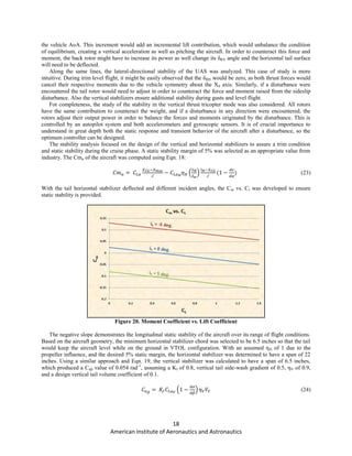
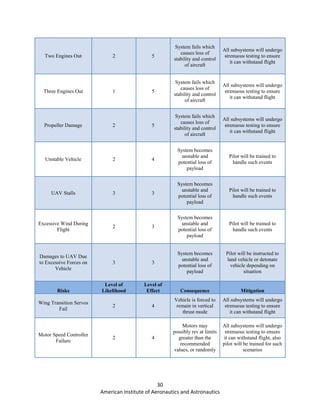
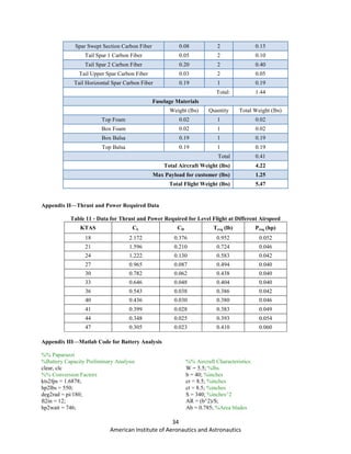
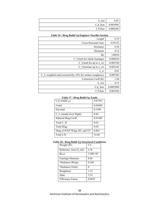
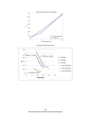
%% Transition Analysis Data
% < < Wings 30 Degrees Up > >
%import .dat file to matlab
[Data,SizeData] =
importfile('transition_wing_30deg_up_0_20_30_35_40_45mph.dat
', 2);
%Substract First Row which to substract Zero offset error
for i = 2:1:SizeData(1)
Data(i,:) = Data(i,:) - Data(1,:);
end
alpha_transition_30deg = Data(2:end,1); %AoA vector in Deg.
Lift_transition_30deg = Data(2:end,2); %Lift Vector in lbs.
Drag_transition_30deg = Data(2:end,3); %Drag Vector in lbs.
Pitch_transition_30deg = Data(2:end,4)*in_2_ft; %Pitching
Moment Vector in lbs*ft
Side_transition_30deg = Data(2:end,5); %Sideforce Vector in lbs
Roll_transition_30deg = Data(2:end,6)*in_2_ft; %Rolling Moment
Vector in lbs*ft
Yaw_transition_30deg = Data(2:end,7)*in_2_ft; %Yawing
Moment Vector in lbs*ft
% < < Wings 60 Degrees Up > >
%import .dat file to matlab
[Data,SizeData] =
importfile('transition_wing_60deg_up_0_20_25_30_35.dat', 2);
%Substract First Row which to substract Zero offset error
for i = 2:1:SizeData(1)
Data(i,:) = Data(i,:) - Data(1,:);
end
alpha_transition_60deg = Data(2:end,1); %AoA vector in Deg.
Lift_transition_60deg = Data(2:end,2); %Lift Vector in lbs.
Drag_transition_60deg = Data(2:end,3); %Drag Vector in lbs.
Pitch_transition_60deg = Data(2:end,4)*in_2_ft; %Pitching
Moment Vector in lbs*ft
Side_transition_60deg = Data(2:end,5); %Sideforce Vector in lbs
Roll_transition_60deg = Data(2:end,6)*in_2_ft; %Rolling Moment
Vector in lbs*ft
Yaw_transition_60deg = Data(2:end,7)*in_2_ft; %Yawing
Moment Vector in lbs*ft
% < < Wings 90 Degrees Up > >
%import .dat file to matlab
[Data,SizeData] =
importfile('transition_wing_90deg_up_0_15_20_25_30.dat', 2);
%Substract First Row which to substract Zero offset error
for i = 2:1:SizeData(1)
Data(i,:) = Data(i,:) - Data(1,:);
end
alpha_transition_90deg = Data(2:end,1); %AoA vector in Deg.
Lift_transition_90deg = Data(2:end,2); %Lift Vector in lbs.
Drag_transition_90deg = Data(2:end,3); %Drag Vector in lbs.
Pitch_transition_90deg = Data(2:end,4)*in_2_ft; %Pitching
Moment Vector in lbs*ft
Side_transition_90deg = Data(2:end,5); %Sideforce Vector in lbs
Roll_transition_90deg = Data(2:end,6)*in_2_ft; %Rolling Moment
Vector in lbs*ft
Yaw_transition_90deg = Data(2:end,7)*in_2_ft; %Yawing
Moment Vector in lbs*ft](https://image.slidesharecdn.com/b6d5ca9f-0cd8-4fef-be65-ca3bfedf9c4c-151130202313-lva1-app6891/85/Paparrazzi_Final-1-56-320.jpg)
![61
American Institute of Aeronautics and Astronautics
Appendix IX—Control Design
Longitundal
%Senior Design - Paparazzi
%Dynamic Stability and Feedback Control
clear
close all
%% Longitudinal State Space
%X(1) = udot
%X(2) = alphadot
%X(3) = thetadot (pitch)
%X(4) = qdot
%X(5) = hdot
% A = [ Xu/m Xw/m 0 -g...
% Zu/(m-Zwdot) Zw/(m-Zwdot) (Zq+m*U0)/(m-
Zwdot) 0...
% (Mu+Zu*Gamma)/Iyy (Mw+Zw*Gamma)/Iyy
((Mq+(Zq+m*U0))*Gamma)/Iyy 0...
% 0 0 1 0]
%B = [
%% Conversion Factors
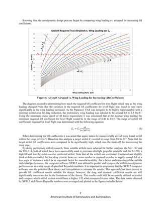
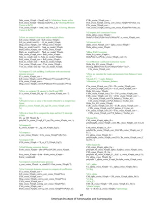
y = 0.0107x - 0.4115
y = 0.0281x - 0.4924
y = 0.0457x - 0.4233
-0.4
-0.3
-0.2
-0.1
0
0.1
0.2
0 5 10 15 20 25
Cm
Speed (kts)
30 Deg.
60 Deg.
90 Deg.](https://image.slidesharecdn.com/b6d5ca9f-0cd8-4fef-be65-ca3bfedf9c4c-151130202313-lva1-app6891/85/Paparrazzi_Final-1-62-320.jpg)
![62
American Institute of Aeronautics and Astronautics
% < < Distance > >
nm_2_miles = 1.15078; %multiply to convert from nm to miles
miles_2_ft = 5280; %multiply to convert from miles to feet
in_2_ft = 1/12; %multiply to convert from in to ft
% < < Speed > >
kts_2_mph = 1.1508; %multiply to convert from kts to mph
kts_2_fps = 1.6878; %multiply to convert from kts to fps
mph_2_fps = 1.46667; %multiply to convert from mph to fps
% < < Mass > >
oz_2_lbs = 1/16; %multiply to convert from oz to lbs
% < < Temperature > >
fah_2_rank = 460.67; %add to convert from Fahrenheit to Rankine
% < < Pressure > >
inHg_2_psf = 70.7262; %multiply to convert from inches Mercury
to Psf
% < < Time > >
hour_2_sec = 3600; %multiply to convert from hours to seconds
min_2_sec = 60; %multiply to convert from min to seconds
% < < Angles > >
deg_2_rad = pi/180; %multiply to convert from degrees to radians
%% Given Constant Atmospheric Data
P_SL = 2116.2; %psf
T_SL = 518.69; %Deg. Rankine
Rho_SL = 0.002377; %slugs/ft3
Gamma_Air = 1.4; %Constant
R_Air = 1716; %Air Constant
mu_Air = 3.7424*10^-7; %Air Constant
delta_STL = 0.9822;
theta_STL_STD = 0.997;
theta_STL_Cold = 0.784;
theta_STL_Hot = 1.0812;
delta_500_STL = 0.9692;
theta_500_STL_STD = 0.994;
theta_500_STL_Cold = 0.7972;
theta_500_STL_Hot = 1.0774;
sigma_500_STL = 0.975;
mu_500_STL = 3.72497*10^-7;
Tatm = T_SL*theta_STL_STD; %Rank
Rair = 1716;
g = 32.2; %gravity constant in ft/sec2
rho = 0.002377*sigma_500_STL; %Density at trim level
mu = (3.62*10^-
7)*((Tatm/518.7)^1.5)*((518.7+198.72)/(Tatm+198.72));
%air viscocity in engineering units at Patm and Tatm
%-> Got equation from Introduction to Flight 7th ed.
nu = mu/rho;
a_SL = 1116; %Speed of Sound at SL in fps
%% Vehicle Geometry
lH = 16.45; %inches
lH = lH*in_2_ft; %ft
cbar_w = 8.5; %in
cbar_w = cbar_w*in_2_ft;
cbar_H = 6.5;
cbar_H = cbar_H*in_2_ft;
alpha0H = 0;
bw = 40;
bw = bw*in_2_ft;
bH = 22;
bH = bH*in_2_ft;
Sw = bw*cbar_w; %Wing Planform Area
SH = bH*cbar_H;
ARw = (bw^2)/Sw;
ARH = (bH^2)/SH;
ht = lH/cbar_w;
hcg = (4*in_2_ft)/cbar_w;
VH = (SH*lH)/(Sw*cbar_w);
etaH = .9; %assumed due to propeller
influence
dTh = 0;
XdTh = 13.5;
XdTh = XdTh*in_2_ft;
M = 5.5/g; %mass of the vehicle
Imat = [4.214*10^6 1.4502*10^3 -2.5678*10^4;... %in
lbs*in^2
1.4502*10^3 4.215*10^6 3.563*10^4;...
-2.5678*10^4 3.563*10^4 2.5144*10^5];
Imat = Imat*(in_2_ft^2)/g; %in slugs*ft^2
Iyy = Imat(2,2); %slugs*ft^2
CD0 = 0.02385; %From Drag build-up Excel File
%% Trim Conditions
U0 = 40; %Trim Speed in fps
U0 = U0*kts_2_fps;
qinf = 0.5*rho*U0^2; %dynamic pressure at trim
qSM = qinf*Sw/M; %Constant in control derivatives
qSCIyy = qinf*Sw*cbar_w/Iyy;
CL0 = g/qSM; %Lift Coefficient at trim
ew = 4.61*(1-0.045*ARw^0.68)-3.1;
ewH = 4.61*(1-0.045*ARH^0.68)-3.1;
CDt = CD0 + (1/(pi*ARw*ew))*CL0^2;
TH_tot = CDt*qinf*Sw;
TH_mot = TH_tot/3;
alpha0 = 0;
Theta_T = 0;
Cm0 = 0.025;
iH = 1.94*deg_2_rad;
%% Stability Derivatives
CTh = TH_mot/(qinf*Sw);](https://image.slidesharecdn.com/b6d5ca9f-0cd8-4fef-be65-ca3bfedf9c4c-151130202313-lva1-app6891/85/Paparrazzi_Final-1-63-320.jpg)
![63
American Institute of Aeronautics and Astronautics
CD_alpha_fun = [0.04584 0.23491]; %1/rad
CD_alpha = polyval(CD_alpha_fun,alpha0);
CD_alphadot = 0.04584;
CLw_alpha = 4.58;
CLH_alpha = 4.12;
CLih = CLH_alpha*(etaH)*(SH/Sw);% + CTh; %Since we
are including (d/dih)(CTh*sin(ih)) which was approx as slope ih.
Cmih = -CLH_alpha*ht*etaH*(SH/Sw);
Cm_alphadot = -32.97; %From wind tunnel
analysis matlab
dE_dalpha = (2*CLw_alpha)/(pi*ARw);
CLH0 = CLH_alpha*(((1-dE_dalpha)*alpha0)+iH-alpha0H);
CDih = (2*CLH_alpha*CLH0*etaH*(SH/Sw))/(pi*ARH*ewH);
Cm_alpha = -0.2406; %1/rad
%Cm_alpha = -0.59;
%% Control Derivatives
Xu_Xpu = qSM*(-1*(((2/U0)*CD0)));
%Xalphadot = -qSM*CD_alphadot;
Xalphadot = 0;
Xalpha = qSM*(CL0-CD_alpha);
Xq = 0;
Xdih = -qSM*CDih;
XdT = qSCIyy*cos(Theta_T)/M;
Zu_Zpu = qSM*(-1*((2/U0)*CL0));
Zalpha = qSM*(CD0-CLw_alpha);
Zq = -VH*CLw_alpha;
Zalphadot = Zq*dE_dalpha;
Zih = -qSM*CLih;
ZdT = -sin(Theta_T)/M;
Mu_Mpu = qSCIyy*((2/U0)*Cm0);
Mq = Zq*hcg;
Malphadot = qSCIyy*Cm_alphadot;
Malpha_Mpalpha = -3.8657; %From Wind Tunnel
analysis 1/rad
Mih = .5*qinf*Sw*Cmih;
MdT = (dTh*cos(Theta_T) - XdTh*sin(Theta_T))/Iyy;
%% State Space
a11 = Xu_Xpu+((Xalphadot*(Zu_Zpu))/(U0-Zalphadot));
a12 = Xalpha+((Xalphadot*Zalpha)/(U0-Zalphadot));
a13 = -g;
a14 = Xq+(Xalphadot*((U0+Zq)/(U0-Zalphadot)));
a15 = 0;
a21 = ((Zu_Zpu)/(U0-Zalphadot));
a22 = Zalpha/(U0-Zalphadot);
a23 = 0;
a24 = ((U0+Zq)/(U0-Zalphadot));
a25 = 0;
a31 = 0;
a32 = 0;
a33 = 0;
a34 = 1;
a35 = 0;
a41 = Mu_Mpu + ((Malphadot*Zu_Zpu)/(U0-Zalphadot));
a42 = Malpha_Mpalpha + ((Malphadot*Zalpha)/(U0-Zalphadot));
a43 = 0;
a44 = Mq + Malphadot*(((U0+Zq)/(U0-Zalphadot)));
a45 = 0;
a51 = 0;
a52 = -U0;
a53 = U0;
a54 = 0;
a55 = 0;
%b11 = Xdih+((Xalphadot*Zih)/(U0-Zalphadot));
b11 = 0;
b12 = XdT+((Xalphadot*ZdT)/(U0-Zalphadot));
b21 = Zih/(U0-Zalphadot);
b22 = ZdT/(U0-Zalphadot);
b31 = 0;
b32 = 0;
b41 = Mih + ((Malphadot*Zih)/(U0-Zalphadot));
b42 = MdT + ((Malphadot*ZdT)/(U0-Zalphadot));
b51 = 0;
b52 = 0;
A = [a11 a12 a13 a14 a15;...
a21 a22 a23 a24 a25;...
a31 a32 a33 a34 a35;...
a41 a42 a43 a44 a45;...
a51 a52 a53 a54 a55];
B = [b11 b21 b31 b41 b51;...
b12 b22 b32 b42 b52]';
% Get the number of states, n, number of controls, m, and the
number of
% outputs, p.
[n,m] = size(B);
C = eye(n,n);
p = size(C,1);
D = zeros(p,m);
% Define the state space model.
sys_ss = ss(A,B,C,D);
% Convert to transfer function.
sys_tf = tf(sys_ss);
% Convert to zero-pole description.
sys_zpk = zpk(sys_ss);
% Convert back to state space
sys_ssa = ss(sys_tf);
%{
%% Simulation of State Space System
% Find the characteristic polynomial.
CharPoly = poly(A);
% Find the system poles.
Poles = roots(CharPoly);
dt = 0.01;
tfinal = 50;
time_s = 0:dt:tfinal;
% Compute the left eigenvectors of A. These are used in tests for
% controllability.
[W,Dc] = eig(A.');
W = conj(W);
% Compute the right eigenvectors of A. These are used in tests for
% observability.
[V,Do] = eig(A);
%% Initial Simulation
t0 = 0:.05:20;
u0(2,1:401) = 0;
u0(1,1:60) = 3.5/57.3;](https://image.slidesharecdn.com/b6d5ca9f-0cd8-4fef-be65-ca3bfedf9c4c-151130202313-lva1-app6891/85/Paparrazzi_Final-1-64-320.jpg)
![64
American Institute of Aeronautics and Astronautics
u0(1,61:120) = 1/57.3;
u0(1,121:180) = 3.5/57.3;
u0(1,181:401) = 0/57.3;
%u0(1,101:401) = 0/57.3;
%{
u0(1,41:80) = 0;
u0(1,81:120) = 1/57.3;
u0(1,121:401) = 0;
%}
x0 = [67.51;0;0;0;400]; %trim
[y1,t1,x1] = lsim(sys_ss,u0,t0,x0);
figure
subplot(5,1,1)
plot(t1,y1(:,1))
xlabel('time (s)')
ylabel('speed (fps)')
title('Surge Velocity vs. time')
subplot(5,1,2)
plot(t1,y1(:,2)*57.3)
xlabel('time (s)')
ylabel('alpha (deg)')
subplot(5,1,3)
plot(t1,y1(:,3)*57.3)
xlabel('time (s)')
ylabel('theta (deg)')
title('Pitch Attitude vs. time')
subplot(5,1,4)
plot(t1,y1(:,4)*57.3)
xlabel('time (s)')
ylabel('Pitch Rate (deg/s)')
subplot(5,1,5)
plot(t1,y1(:,5))
xlabel('time (s)')
ylabel('Altitude (ft)')
figure
plot(t1,u0(1,:)*57.3)
xlabel('time (sec)')
ylabel('Tail Incidence Angle (deg.)')
%}
%% System for Control
Acc = A(1:4,1:4);
Bcc = B(1:4,1:2);
%Bcc = B(1:4,1);
[nc,mc] = size(Bcc);
Ccc = eye(nc,nc);
pcc = size(Ccc,1);
Dcc = zeros(pcc,mc);
% Define the state space model.
sys_cc = ss(Acc,Bcc,Ccc,Dcc);
% Convert to transfer function.
sys_tf = tf(sys_cc);
% Convert to zero-pole description.
sys_zpk = zpk(sys_cc);
% Convert back to state space
sys_ssa = ss(sys_tf);
% Find the characteristic polynomial.
CharPoly = poly(Acc);
% Find the system poles.
Poles = roots(CharPoly);
% Compute the left eigenvectors of A. These are used in tests for
% controllability.
[W,Dc] = eig(Acc.');
W = conj(W);
% Compute the right eigenvectors of A. These are used in tests for
% observability.
[V,Do] = eig(Acc);
% Damping characteristics
damp(Acc)
% Compute the controllability matrix, P, using the MATLAB
function.
P = ctrb(sys_cc);
% Determine if the system is controllable by checking the rank of
P.
% The rank of P should match the number of rows (or columns) of
the square
% matrix A.
if rank(P) == nc
disp('The system is controllable.');
else
disp('The system is NOT controllable.');
end
disp(' ');
% Compute the condition number for impending singularity.
Cn = cond(Acc);
% Degree of Controllability between Mode i and Control j.
DoC = zeros(nc,mc);
for i = 1:nc
for j = 1:mc
DoC(i,j) = abs(dot(Bcc(:,j),
W(i,:))/norm(Bcc(:,j))/norm(W(i,:)));
end
end
% Compute the inverse matrix Pccfi.
Pccfi = zeros(nc,nc);
base = CharPoly(nc:-1:2);
for i = nc:-1:1
if i == nc
% Last row. Set the first element to 1.
Pccfi(i,1) = 1;
else
% Populate the ith row
Pccfi(i,1:nc-i+1) = [base(i:end) 1];
end
end
%{
% Compute the Transformation matrix, Tccf.
Tccf = P*Pccfi;
% Compute the CCF matrices.
Accf = TccfAcc*Tccf;
Bccf = TccfBcc;
Cccf = Ccc*Tccf;
Dccf = Dcc;](https://image.slidesharecdn.com/b6d5ca9f-0cd8-4fef-be65-ca3bfedf9c4c-151130202313-lva1-app6891/85/Paparrazzi_Final-1-65-320.jpg)
![65
American Institute of Aeronautics and Astronautics
%}
% Compute the observability matrix, Q, using the MATLAB
function.
Q = obsv(sys_cc);
% Determine if the system is observable by checking the rank of
Q.
% The rank of Q should match the number of rows (or columns) of
the square
% matrix A.
if rank(Q) == nc
disp('The system is observable.');
else
disp('The system is NOT observable.');
end
disp(' ');
% Degree of Observability between Mode i and Measurement j.
DoO = zeros(pcc,nc);
for j = 1:pcc
for i = 1:nc
DoO(j,i) = abs(dot(Ccc(j,:),
V(:,i))/norm(Ccc(j,:))/norm(V(:,i)));
end
end
% Perform a stability analysis using Lyapunov stability.
disp('Lyapunov Stability Analysis.');
% Find the poles with zero real part.
i_zero_real = find(real(Poles) == 0);
if ~isempty(i_zero_real)
% Lyapunov stabilty analysis will not work if there is at least
one
% pole with zero real part. At this point, we can only check for
% marginally stable or unstable systems.
else
% Lyapunov stability analysis will work.
% Form a positive definite matrix, Q.
Qc = eye(nc);
% Solve the Lyapunov equation for P.
Pc = lyap(Acc',Qc);
% Perform Sylvester's Method to determine if P is positive
definite.
pm = zeros(1,nc);
for i = 1:nc
pm(i) = det(Pc(1:i,1:i));
end
if all(pm > 0)
disp('P is positive definite. System is asymptotically stable.');
elseif any(pm < 0)
disp('P is not positive definite. System is unstable.');
else
disp('P is positive semi-definite. Try another Q.');
end
end
% Determine a desired response for the system. Two approaches
are
% investigated: (1.) second order dominant; (2.) 6th order ITAE.
% Specify the overshoot percentage and settling time.
PO = 5;
ts = 1.5;
% Determine damping ratio from PO and natural frequency from
settling time
% and zeta.
term = pi^2 + log(PO/100)^2;
zeta = abs(log(PO/100))/sqrt(term);
wn = 4/(zeta*ts);
% Desired 2nd order system.
num2 = wn^2;
den2 = [1 2*zeta*wn wn^2];
Des2 = tf(num2,den2);
% Dominant 2nd order eigenvalues.
DesEig2 = roots(den2);
% Get the stepinfo
stepinfo(Des2)
% Augment with 2 additional poles.
Aug4 = zeros(2,1);
Aug4(1) = 10*real(DesEig2(1));
Aug4(2) = Aug4(1)-1;
% 4th order transfer function with augmented poles,
den_Aug4 = conv(den2,conv([1 -Aug4(1)],([1 -Aug4(2)])));
Aug2 = tf(num2, den_Aug4);
% Plot the dominant 2nd order response.
figure
step(Des2, 'b-', Aug2*den_Aug4(end)/num2, 'g--');grid on
legend('Desired 2nd', 'Augmented 2nd order');
% Compute the state feedback regulator based upon the augmented
2nd order
% system.
K = place(Acc,Bcc,[DesEig2;Aug4]);
% Form plant system. Set output matrix for state feedback control.
sys_p.Ap = Acc;
sys_p.Bp = Bcc;
sys_p.Cp = eye(nc);
sys_p.Dp = zeros(nc,mc);
% Form controller system.
sys_c.Ac = 0;
sys_c.Bc1= 0;
sys_c.Bc2= 0;
sys_c.Cc = 0;
sys_c.Dc1= -K;
sys_c.Dc2= zeros(mc,mc);
% Form closed loop system.
[Acl,Bcl,Ccl,Dcl] = closed_loop_system(sys_p, sys_c);
sys_cl = ss(Acl,Bcl,Ccl,Dcl);
%% Simulation
t = 0:.05:200;
x0 = [0;0;1.5/57.3;0]; %trim
% Closed-loop response (zero input, ICs).
[Yo,t,Xo] = lsim(sys_cc,zeros(numel(t),mc),t,x0);
[Yc,t,Xc] = lsim(sys_cl,zeros(numel(t),mc),t,x0);](https://image.slidesharecdn.com/b6d5ca9f-0cd8-4fef-be65-ca3bfedf9c4c-151130202313-lva1-app6891/85/Paparrazzi_Final-1-66-320.jpg)
![66
American Institute of Aeronautics and Astronautics
figure
plot(Xo(:,3)*57.3,Xo(:,4)*57.3)
grid on
xlabel('theta, deg.')
ylabel('dtheta / dt, deg./s')
title('Phase Diagram for Pitch Attitude')
% Control signals.
u = zeros(numel(t),mc);
for i = 1:mc
for j = 1:numel(t)
u(j,i) = -K(i,:)*Xc(j,:)';
end
end
% Plot the control signals.
figure
%subplot(2,1,1);
plot(t, u(:,1)*57.3);grid on
xlabel('Time, s');
ylabel('di_t (deg.)');
title('Regulating controls vs. Time');
%{
subplot(2,1,2);
plot(t, u(:,2));grid on
xlabel('Time, s');
ylabel('dThrust, N');
%}
% Open-loop and closed loop plots of the model states.
figure
subplot(4,1,1);
plot(t,Xo(:,1),'--b',t,Xc(:,1),'-r');grid on
xlabel('Time, s');
ylabel('speed, fps');
title('Model States vs. Time with 0 input and I.C.s')
subplot(4,1,2);
plot(t,Xo(:,2)*57.3,'--b',t,Xc(:,2)*57.3,'-r');grid on
xlabel('Time, s');
ylabel('alpha , rad');
subplot(4,1,3);
plot(t,Xo(:,3)*57.3,'--b',t,Xc(:,3)*57.3,'-r');grid on
xlabel('Time, s');
ylabel('theta , rad');
subplot(4,1,4);
plot(t,Xo(:,4)*57.3,'--b',t,Xc(:,4)*57.3,'-r');grid on
xlabel('Time, s');
ylabel('pitch rate, rad/s');
legend('Uncontrolled Response','Controlled
Response','Location','NorthEast')
Acl2 = zeros(n,n);
Acl2(1:4,1:4) = Acl;
Acl2(5,:) = A(5,:);
sys_cl2 = ss(Acl2,B,C,D);
t0 = 0:.05:10;
%{%}
u0(2,1:401) = 0;
u0(1,1:60) = 0/57.3;
u0(1,61:100) = 1.5/57.3;
u0(1,101:180) = 0/57.3;
u0(1,181:220) = -1.5/57.3;
u0(1,221:401) = 0/57.3;
u01 = 1/57.3*ones(numel(t0),1);
u02 = 0*ones(numel(t0),1);
u03 = 1*ones(numel(t0),1);
xx0 = [0;0;0;0;400]; %trim
[y1,t1,x1] = lsim(sys_cl2,[u01 u02],t0,xx0);
[y2,t2,x2] = lsim(sys_ss,[u01 u02],t0,xx0);
[y3,t3,x3] = lsim(sys_cl2,[u02 u03],t0,xx0);
[y4,t4,x4] = lsim(sys_ss,[u02 u03],t0,xx0);
figure
subplot(5,1,1)
plot(t1,y1(:,1),'-r')
hold on
plot(t1,y2(:,1),'--b')
xlabel('time (s)')
ylabel('speed (fps)')
title('Surge Velocity vs. time')
subplot(5,1,2)
plot(t1,y1(:,2)*57.3,'-r')
hold on
plot(t1,y2(:,2)*57.3,'--b')
xlabel('time (s)')
ylabel('alpha (deg)')
subplot(5,1,3)
plot(t1,y1(:,3)*57.3,'-r')
hold on
plot(t1,y2(:,3)*57.3,'--b')
xlabel('time (s)')
ylabel('theta (deg)')
title('Pitch Attitude vs. time')
subplot(5,1,4)
plot(t1,y1(:,4)*57.3,'-r')
hold on
plot(t1,y2(:,4)*57.3,'--b')
xlabel('time (s)')
ylabel('Pitch Rate (deg/s)')
title('Pitch Rate vs. time')
subplot(5,1,5)
plot(t1,y1(:,5),'-r')
hold on
plot(t1,y2(:,5),'--b')
xlabel('time (s)')
ylabel('Altitude (ft)')
title('Model State vs. Time with 0 I.C.s and Tail Incidence step
input')
legend('Controlled Response','Uncontrolled Response')
figure
subplot(5,1,1)
plot(t1,y3(:,1),'-r')
hold on
plot(t1,y4(:,1),'--b')
xlabel('time (s)')
ylabel('speed (fps)')
title('Surge Velocity vs. time')
subplot(5,1,2)
plot(t1,y3(:,2)*57.3,'-r')
hold on
plot(t1,y4(:,2)*57.3,'--b')
xlabel('time (s)')
ylabel('alpha (deg)')
subplot(5,1,3)
plot(t1,y3(:,3)*57.3,'-r')
hold on
plot(t1,y4(:,3)*57.3,'--b')
xlabel('time (s)')
ylabel('theta (deg)')
title('Pitch Attitude vs. time')
subplot(5,1,4)](https://image.slidesharecdn.com/b6d5ca9f-0cd8-4fef-be65-ca3bfedf9c4c-151130202313-lva1-app6891/85/Paparrazzi_Final-1-67-320.jpg)
![67
American Institute of Aeronautics and Astronautics
plot(t1,y3(:,4)*57.3,'-r')
hold on
plot(t1,y4(:,4)*57.3,'--b')
xlabel('time (s)')
ylabel('Pitch Rate (deg/s)')
title('Pitch Rate vs. time')
subplot(5,1,5)
plot(t1,y3(:,5),'-r')
hold on
plot(t1,y4(:,5),'--b')
xlabel('time (s)')
ylabel('Altitude (ft)')
title('Model State vs. Time with 0 I.C.s and Thrust step input')
legend('Controlled Response','Uncontrolled Response')
t6 = 0:length(u0)-1;
%{%}
figure
plot(t6,u0(1,:)*57.3)
xlabel('time (sec)')
ylabel('Tail Incidence Angle (deg.)')
[y5,t6,x5] = lsim(sys_cl2,u0,t6,xx0);
[y6,t6,x6] = lsim(sys_ss,u0,t6,xx0);
figure
subplot(1,2,1)
plot(t6,y5(:,5),'-r')
hold on
plot(t6,y6(:,5),'--b')
xlabel('time (s)')
ylabel('Altitude (ft)')
subplot(1,2,2)
plot(t6,u0(1,:)*57.3)
xlabel('time (sec)')
ylabel('Tail Incidence Angle (deg.)')
title('Altitude vs. Time with Tail Incidence Control')
%%%%% SERVO MECHANISM TRACKING %%%%%
% Track outputs y1, y2 and y3.
CC = zeros(2,5);
CC(1,:) = C(1,:);
%CC(2,:) = C(3,:);
CC(2,:) = C(5,:);
Csv = CC;
p = 3;
% Matrices
Asv = zeros(n+m, n+m);
Asv(1:n,1:n) = A;
Asv(n+1:end,1:n) = -Csv;
Bsv = zeros(n+m, m);
Bsv(1:n,:) = B;
% Gain design. Add 3 additional eigenvalues for each reference.
Ksv = place(Asv,Bsv,[DesEig2;Aug4;-6;-12;-7]);
Kv = Ksv(:,1:n);
kI = -Ksv(:,n+1:end);
% Closed loop system
% Aclsv = [A-B*Kv, B*kI;-Csv, zeros(p,m)];
% Bclsv = [zeros(n,m);eye(m)];
% Cclsv = [Csv, zeros(m,m)];
% Dclsv = 0;
% sys_clsv = ss(Aclsv,Bclsv,Cclsv,Dclsv);
% Form plant system. Set output matrix for state feedback control.
sys_p.Ap = A;
sys_p.Bp = B;
sys_p.Cp = eye(n);
sys_p.Dp = zeros(n,m);
% Form controller system. Tracking on each of the three position
states.
sys_c.Ac = zeros(m,m);
sys_c.Bc1= -CC;
sys_c.Bc2= eye(m);
sys_c.Cc = kI;
sys_c.Dc1= -Kv;
sys_p.Dc2= zeros(n,m);
% Form closed loop system.
[Aclsv, Bclsv, Cclsv, Dclsv] = closed_loop_system(sys_p, sys_c);
sys_clsv = ss(Aclsv,Bclsv,Cclsv,Dclsv);
% Simulation
dt = 0.01;
tfinal = 10;
t = 0:dt:tfinal;
% Simulation #1: r1 = 1, r2 = 1 and r3 = 1. Zero I.C.
r1 = ones(numel(t),1);
r2 = ones(numel(t),1);
%r3 = ones(numel(t),1);
[y_clsv,time_clsv,x_clsv] = lsim(sys_clsv,[r1, r2],t);
% Control signals.
u = zeros(numel(t),m);
for i = 1:m
for j = 1:numel(t)
u(j,i) = -Kv(i,:)*x_clsv(j,1:n)'+kI(i,:)*x_clsv(j,n+1:end)';
end
end
% Plot the control signals.
figure
subplot(2,1,1);
plot(t, u(:,1)*57.3);grid on
xlabel('Time, s');
ylabel('delta_{tail}, deg.');
title('Tracking controls vs. Time');
subplot(2,1,2);
plot(t, u(:,2)/38);grid on
xlabel('Time, s');
ylabel('delta_{thrust}, lbf');
% Plot output responses.
figure
subplot(3,1,1);
plot(time_clsv, y_clsv(:,1),'b-');grid on
xlabel('Time, s');
ylabel('y_1, m');
title('Unit step responses for each output vs. Time');
subplot(3,1,2);
plot(time_clsv, y_clsv(:,2),'b-');grid on
xlabel('Time, s');
ylabel('y_2, m');
subplot(3,1,3);
plot(time_clsv, y_clsv(:,3),'b-');grid on
xlabel('Time, s');
ylabel('y_3, m');
figure
subplot(3,1,1);
plot(time_clsv, x_clsv(:,1),'b-');grid on](https://image.slidesharecdn.com/b6d5ca9f-0cd8-4fef-be65-ca3bfedf9c4c-151130202313-lva1-app6891/85/Paparrazzi_Final-1-68-320.jpg)
![68
American Institute of Aeronautics and Astronautics
xlabel('Time, s');
ylabel('speed, fps');
title('Unit step responses for each output vs. Time');
subplot(3,1,2);
plot(time_clsv, x_clsv(:,3)*57.3,'b-');grid on
xlabel('Time, s');
ylabel('theta, deg.');
subplot(3,1,3);
plot(time_clsv, x_clsv(:,5),'b-');grid on
xlabel('Time, s');
ylabel('altitude, ft');
%%%%% FREQUENCY ANALYSIS %%%%%
% Perform frequency analysis of servo tracker.
w = logspace(0,4,400);
freq_resp1 = freq_analysis(sys_p, sys_c, w, 1, 3);
freq_resp2 = freq_analysis(sys_p, sys_c, w, 2, 3);
% Plot frequency data.
%plot_freq_resp(freq_resp1, w);
%plot_freq_resp(freq_resp2, w);
%% Altitude Autopilot Control
%% Comparison of Elevator input Controlled/Uncontrolled
%{%}
Hmax = 500;
Hc = zeros(312,1);
Hc(:,1)=[zeros(10,1);Hmax/100*[0:1:100]';Hmax*ones(50,1);Hma
x/100*[100:-1:0]';zeros(50,1)];
t4 = 0:length(Hc)-1;
%{
[Yh,t4]=lsim(sys_cl2(:,2),Hc,t4);
[Yh2,t4]=lsim(sys_ss(:,2),Hc,t4);
%}
%{%}
[Yh,t4]=lsim(sys_cl2(:,2),Hc,t4);
[Yh2,t4]=lsim(sys_ss(:,2),Hc,t4);
figure
subplot(5,1,1)
plot(t4,Yh(:,1),'-r')
hold on
plot(t4,Yh2(:,1),'--b')
xlabel('time, sec')
ylabel('Velocity, fps')
subplot(5,1,2)
plot(t4,Yh(:,2),'-r')
hold on
plot(t4,Yh2(:,2),'--b')
xlabel('time, sec')
ylabel('alpha, deg.')
subplot(5,1,3)
plot(t4,Yh(:,3),'-r')
hold on
plot(t4,Yh2(:,3),'--b')
xlabel('time, sec')
ylabel('theta, deg.')
subplot(5,1,4)
plot(t4,Yh(:,4),'-r')
hold on
plot(t4,Yh2(:,4),'--b')
xlabel('time, sec')
ylabel('dtheta/dt, deg./sec')
subplot(5,1,5)
plot(t4,Yh(:,5),'-r')
hold on
plot(t4,Yh2(:,5),'--b')
xlabel('time, sec')
ylabel('Altitude, ft.')
%% simplified model
Ashort = A(2:4,2:4);
Bshort = B(2:4,1:2);
Ashort = [Ashort(1,1) Ashort(1,3);Ashort(3,1) Ashort(3,3)];
Bshort = [Bshort(1,1) Bshort(3,1)]';
Cshort = eye(2);
Dshort = zeros(2,1);
sys_short = ss(Ashort, Bshort, Cshort, Dshort);
CPshort = poly(Ashort);
% Calculate the open-loop system eigenvalues, zeta and wn from
ABCD
[wn0_short,zeta0_short,Eigs0_short] = damp(Ashort);
% Convert to transfer function.
sys_tf_short = tf(sys_short);
time_short = 0:0.001:3.0;
x0sh = [0; 0];
u = zeros(size(time_short));
u(1:500) = -1/57.3;
[Y0sh,t_short,X0sh] = lsim(sys_short,u,time_short,x0sh);
Tp_short = (2*pi)/(wn0_short(1)); %Seconds
T_Half_short = -log(2)/(real(Eigs0_short(1))); %Seconds
figure
plot(t_short,X0sh(:,1)*57.3,'-b','LineWidth',2)
xlabel('time (sec)')
ylabel('alpha (deg.)')
title('Short Period Response to alpha = 0.5 deg. Disturbance')
%% SImulation
[Vsh2, Gamsh2] = eig(A);
xshort = real(Vsh2(:,2));
xphug = real(Vsh2(:,4));
xshort = xshort/norm(xshort);
xphug = xphug/norm(xphug);
Nsamp = 100;
yshort = zeros(5,Nsamp);
timesh = linspace(0,3,Nsamp);
for i = 1:Nsamp
yshort(:,i) = C*expm(timesh(i)*A)*xshort;
end
figure
subplot(3,2,1)
plot(timesh,yshort(1,:))
ylabel('speed (fps)')
xlabel('time (sec)')
title('Short Period Responses')](https://image.slidesharecdn.com/b6d5ca9f-0cd8-4fef-be65-ca3bfedf9c4c-151130202313-lva1-app6891/85/Paparrazzi_Final-1-69-320.jpg)
![69
American Institute of Aeronautics and Astronautics
subplot(3,2,2)
plot(timesh,yshort(2,:)/deg_2_rad)
ylabel('alpha (deg)')
xlabel('time (sec)')
subplot(3,2,3)
plot(timesh,yshort(3,:)/deg_2_rad)
ylabel('q (deg./sec)')
xlabel('time (sec)')
subplot(3,2,4)
plot(timesh,yshort(4,:)/deg_2_rad)
ylabel('theta (deg)')
xlabel('time (sec)')
subplot(3,2,5)
plot(timesh,yshort(5,:))
ylabel('altitude (ft)')
xlabel('time (sec)')
h1=zeros(5,Nsamp); h2=zeros(5,Nsamp);
for i=1:Nsamp,
h1(:,i)=C*expm(timesh(i)*A)*B(:,1); % impulse response from
u_w
h2(:,i)=C*expm(timesh(i)*A)*B(:,2); % imp resp from v_w
end
figure
subplot(3,2,1)
plot(timesh,h1(1,:))
ylabel('speed (fps)')
xlabel('time (sec)')
title('Impulse Responses to Wing Incidence')
subplot(3,2,2)
plot(timesh,h1(2,:)/deg_2_rad)
ylabel('alpha (deg)')
xlabel('time (sec)')
subplot(3,2,3)
plot(timesh,h1(3,:)/deg_2_rad)
ylabel('theta (deg)')
xlabel('time (sec)')
subplot(3,2,4)
plot(timesh,h1(4,:)/deg_2_rad)
ylabel('q (deg./sec)')
xlabel('time (sec)')
subplot(3,2,5)
plot(timesh,h1(5,:))
ylabel('altitude (ft)')
xlabel('time (sec)')
figure
subplot(3,2,1)
plot(timesh,h2(1,:))
ylabel('speed (fps)')
xlabel('time (sec)')
title('Impulse Responses to Change in Thrust')
subplot(3,2,2)
plot(timesh,h2(2,:)/deg_2_rad)
ylabel('alpha (deg)')
xlabel('time (sec)')
subplot(3,2,3)
plot(timesh,h2(3,:)/deg_2_rad)
ylabel('theta (deg)')
xlabel('time (sec)')
subplot(3,2,4)
plot(timesh,h2(4,:)/deg_2_rad)
ylabel('q (deg./sec)')
xlabel('time (sec)')
subplot(3,2,5)
plot(timesh,h2(5,:))
ylabel('altitude (ft)')
xlabel('time (sec)')
%% Phugoid
Nsamp = 1000; %number of time samples
yphug=zeros(5,Nsamp);
tphug=linspace(0,1000,Nsamp);
for i=1:Nsamp
yphug(:,i)=C*expm(tphug(i)*A)*xphug;
end
figure
subplot(3,2,1)
plot(tphug,yphug(1,:))
ylabel('speed (fps)')
xlabel('time (sec)')
title('Phugoid Motion')
subplot(3,2,2)
plot(tphug,yphug(2,:)/deg_2_rad)
ylabel('alpha (deg)')
xlabel('time (sec)')
subplot(3,2,3)
plot(tphug,yphug(3,:))
ylabel('q_{inf} (psf)')
xlabel('time (sec)')
subplot(3,2,4)
plot(tphug,yphug(4,:)/deg_2_rad)
ylabel('theta (deg)')
xlabel('time (sec)')
subplot(3,2,5)
plot(tphug,yphug(5,:))
ylabel('altitude (ft)')
xlabel('time (sec)')
figure
plot(tphug,yphug(1,:),'-r','LineWidth',2)
hold on
plot(tphug,yphug(5,:),'--b','LineWidth',2)
xlabel('time (sec)')
ylabel('Amplitude')
title('Phugoid Mode')
legend('Speed','Altitude','Location','NorthEast')
axis([0 100 -1 1])
% Calculate the open-loop system eigenvalues, zeta and wn from
ABCD
[wn0,zeta0,Eigs0] = damp(A);
Eigs_phug = Eigs0(4:5);
Damp_phug = zeta0(4:5);
wn_phug = wn0(4:5);
Tp_phug = (2*pi)/(wn_phug(1)); %Seconds
T_Half_phug = -log(2)/(real(Eigs_phug(1))); %Seconds
Lateral
%Senior Design - Paparazzi
%Dynamic Stability and Feedback Control
clear
close all](https://image.slidesharecdn.com/b6d5ca9f-0cd8-4fef-be65-ca3bfedf9c4c-151130202313-lva1-app6891/85/Paparrazzi_Final-1-70-320.jpg)
![70
American Institute of Aeronautics and Astronautics
%% Longitudinal State Space
%X(1) = Beta (Sideslip Angle)
%X(2) = Phi (Bank Angle)
%X(3) = p (roll rate)
%X(4) = r (yaw rate)
%X(5) = psy (Heading Angle)
% A = [ Xbet/U0 g/U0 Yp/U0 (Yr/U0 -1) 0...
% 0 0 1 0 0...
% Lbet 0 Lp Lr 0...
% Nbet 0 Np Nr 0...
% 0 0 0 1 0]
%B = [
%% Conversion Factors
% < < Distance > >
nm_2_miles = 1.15078; %multiply to convert from nm to miles
miles_2_ft = 5280; %multiply to convert from miles to feet
in_2_ft = 1/12; %multiply to convert from in to ft
% < < Speed > >
kts_2_mph = 1.1508; %multiply to convert from kts to mph
kts_2_fps = 1.6878; %multiply to convert from kts to fps
mph_2_fps = 1.46667; %multiply to convert from mph to fps
% < < Mass > >
oz_2_lbs = 1/16; %multiply to convert from oz to lbs
% < < Temperature > >
fah_2_rank = 460.67; %add to convert from Fahrenheit to Rankine
% < < Pressure > >
inHg_2_psf = 70.7262; %multiply to convert from inches Mercury
to Psf
% < < Time > >
hour_2_sec = 3600; %multiply to convert from hours to seconds
min_2_sec = 60; %multiply to convert from min to seconds
% < < Angles > >
deg_2_rad = pi/180; %multiply to convert from degrees to radians
%% Given Constant Atmospheric Data
P_SL = 2116.2; %psf
T_SL = 518.69; %Deg. Rankine
Rho_SL = 0.002377; %slugs/ft3
Gamma_Air = 1.4; %Constant
R_Air = 1716; %Air Constant
mu_Air = 3.7424*10^-7; %Air Constant
delta_STL = 0.9822;
theta_STL_STD = 0.997;
theta_STL_Cold = 0.784;
theta_STL_Hot = 1.0812;
delta_500_STL = 0.9692;
theta_500_STL_STD = 0.994;
theta_500_STL_Cold = 0.7972;
theta_500_STL_Hot = 1.0774;
sigma_500_STL = 0.975;
mu_500_STL = 3.72497*10^-7;
Tatm = T_SL*theta_STL_STD; %Rank
Rair = 1716;
g = 32.2; %gravity constant in ft/sec2
rho = 0.002377*sigma_500_STL; %Density at trim level
mu = (3.62*10^-
7)*((Tatm/518.7)^1.5)*((518.7+198.72)/(Tatm+198.72));
%air viscocity in engineering units at Patm and Tatm
%-> Got equation from Introduction to Flight 7th ed.
nu = mu/rho;
a_SL = 1116; %Speed of Sound at SL in fps
%% Vehicle Geometry
lH = 16.45; %inches
lH = lH*in_2_ft; %ft
cbar_w = 8.5; %in
cbar_w = cbar_w*in_2_ft;
cbar_H = 6.5;
cbar_H = cbar_H*in_2_ft;
alpha0H = 0;
bw = 40;
bw = bw*in_2_ft;
bH = 22;
bH = bH*in_2_ft;
Sw = bw*cbar_w; %Wing Planform Area
SH = bH*cbar_H;
ARw = (bw^2)/Sw;
ARH = (bH^2)/SH;
ht = lH/cbar_w;
hcg = (4*in_2_ft)/cbar_w;
VH = (SH*lH)/(Sw*cbar_w);
etaH = .9; %assumed due to propeller
influence
dTh = 0;
XdTh = 13.5;
XdTh = XdTh*in_2_ft;
M = 5.5/g; %mass of the vehicle
Imat = [4.214*10^6 1.4502*10^3 -2.5678*10^4;... %in
lbs*in^2
1.4502*10^3 4.215*10^6 3.563*10^4;...
-2.5678*10^4 3.563*10^4 2.5144*10^5];
Imat = Imat*(in_2_ft^2)/g; %in slugs*ft^2
Iyy = Imat(2,2); %slugs*ft^2
CD0 = 0.02385; %From Drag build-up Excel File
%% Trim Conditions
U0 = 40; %Trim Speed in fps
U0 = U0*kts_2_fps;
qinf = 0.5*rho*U0^2; %dynamic pressure at trim](https://image.slidesharecdn.com/b6d5ca9f-0cd8-4fef-be65-ca3bfedf9c4c-151130202313-lva1-app6891/85/Paparrazzi_Final-1-71-320.jpg)
![71
American Institute of Aeronautics and Astronautics
qSM = qinf*Sw/M; %Constant in control derivatives
qSCIyy = qinf*Sw*cbar_w/Iyy;
CL0 = g/qSM; %Lift Coefficient at trim
ew = 4.61*(1-0.045*ARw^0.68)-3.1;
ewH = 4.61*(1-0.045*ARH^0.68)-3.1;
CDt = CD0 + (1/(pi*ARw*ew))*CL0^2;
TH_tot = CDt*qinf*Sw;
TH_mot = TH_tot/3;
alpha0 = 0;
Theta_T = 0;
%% Stability Derivatives
Cn_bet = 0.0019*180/pi; %1/rad
CL_bet = 0;
CL_p = -0.245;
CL_r = -0.0012;
CL_dw = 0.0032*180/pi;
%Cn_p = -0.0016;
Cn_p = -0.00;
Cn_r = -0.3234;
%Cn_r = -0.3234;
Cn_dw = 0.0027*180/pi;
CTh = TH_mot/(qinf*Sw);
%% Control Derivatives
Y_bet = qSM*Cn_bet;
Y_p = 0;
Y_r = 0;
L_bet = (qinf*Sw*bw/Imat(1,1))*CL_bet;
L_p = (qinf*Sw*bw/Imat(1,1))*CL_p;
L_r = (qinf*Sw*bw/Imat(1,1))*CL_r;
L_dr = 0;
L_dw =(qinf*Sw*bw/Imat(1,1))*(CL_dw + (2*CTh/pi));
N_bet = (qinf*Sw*bw/Imat(3,3))*Cn_bet;
N_p = (qinf*Sw*bw/Imat(3,3))*Cn_p;
N_r = (qinf*Sw*bw/Imat(3,3))*Cn_r;
N_dr = (qinf*Sw*bw/Imat(3,3))*(2*CTh/pi)*ht;
N_dw = (qinf*Sw*bw/Imat(3,3))*(Cn_dw+ (2*CTh/pi));
Ydr = qSM*(2*CTh/pi);
%% State Space
a11 = Y_bet/U0;
a12 = g/U0;
a13 = 0;
a14 = -1;
a15 = 0;
a21 = 0;
a22 = 0;
a23 = 1;
a24 = 0;
a25 = 0;
a31 = (L_bet+(N_bet*Imat(1,3)/Imat(1,1)))/(1-
((Imat(1,3)^2)/(Imat(1,1)*Imat(3,3))));
a32 = 0;
a33 = (L_p+(N_p*Imat(1,3)/Imat(1,1)))/(1-
((Imat(1,3)^2)/(Imat(1,1)*Imat(3,3))));
a34 = (L_r+(N_r*Imat(1,3)/Imat(1,1)))/(1-
((Imat(1,3)^2)/(Imat(1,1)*Imat(3,3))));
a35 = 0;
a41 = (N_bet+(L_bet*Imat(1,3)/Imat(3,3)))/(1-
((Imat(1,3)^2)/(Imat(1,1)*Imat(3,3))));
a42 = 0;
a43 = (N_p+(L_p*Imat(1,3)/Imat(3,3)))/(1-
((Imat(1,3)^2)/(Imat(1,1)*Imat(3,3))));
a44 = (N_r+(L_r*Imat(1,3)/Imat(3,3)))/(1-
((Imat(1,3)^2)/(Imat(1,1)*Imat(3,3))));
a45 = 0;
a51 = 0;
a52 = 0;
a53 = 0;
a54 = 1;
a55 = 0;
b11 = 0;
b12 = Ydr/U0;
b21 = 0;
b22 = 0;
b31 = (L_dw+(N_dw*Imat(1,3)/Imat(1,1)))/(1-
((Imat(1,3)^2)/(Imat(1,1)*Imat(3,3))));
b32 = (L_dr+(N_dr*Imat(1,3)/Imat(1,1)))/(1-
((Imat(1,3)^2)/(Imat(1,1)*Imat(3,3))));
b41 = (N_dw+(L_dw*Imat(1,3)/Imat(3,3)))/(1-
((Imat(1,3)^2)/(Imat(1,1)*Imat(3,3))));
b42 = (N_dr+(L_dr*Imat(1,3)/Imat(3,3)))/(1-
((Imat(1,3)^2)/(Imat(1,1)*Imat(3,3))));
b51 = 0;
b52 = 0;
A = [a11 a12 a13 a14 a15;...
a21 a22 a23 a24 a25;...
a31 a32 a33 a34 a35;...
a41 a42 a43 a44 a45;...
a51 a52 a53 a54 a55];
damp(A)
B = [b11 b21 b31 b41 b51;...
b12 b22 b32 b42 b52]';
% Get the number of states, n, number of controls, m, and the
number of
% outputs, p.
[n,m] = size(B);
C = eye(n,n);
p = size(C,1);
D = zeros(p,m);
% Define the state space model.
sys_ss = ss(A,B,C,D);
% Convert to transfer function.
sys_tf = tf(sys_ss);
% Convert to zero-pole description.
sys_zpk = zpk(sys_ss);
% Convert back to state space
sys_ssa = ss(sys_tf);](https://image.slidesharecdn.com/b6d5ca9f-0cd8-4fef-be65-ca3bfedf9c4c-151130202313-lva1-app6891/85/Paparrazzi_Final-1-72-320.jpg)
![72
American Institute of Aeronautics and Astronautics
%{
%% Simulation of State Space System
% Find the characteristic polynomial.
CharPoly = poly(A);
% Find the system poles.
Poles = roots(CharPoly);
dt = 0.01;
tfinal = 50;
time_s = 0:dt:tfinal;
% Compute the left eigenvectors of A. These are used in tests for
% controllability.
[W,Dc] = eig(A.');
W = conj(W);
% Compute the right eigenvectors of A. These are used in tests for
% observability.
[V,Do] = eig(A);
%% Initial Simulation
t0 = 0:.05:20;
u0(2,1:401) = 0;
u0(1,1:60) = 3.5/57.3;
u0(1,61:120) = 1/57.3;
u0(1,121:180) = 3.5/57.3;
u0(1,181:401) = 0/57.3;
%u0(1,101:401) = 0/57.3;
%{
u0(1,41:80) = 0;
u0(1,81:120) = 1/57.3;
u0(1,121:401) = 0;
%}
x0 = [67.51;0;0;0;400]; %trim
[y1,t1,x1] = lsim(sys_ss,u0,t0,x0);
figure
subplot(5,1,1)
plot(t1,y1(:,1))
xlabel('time (s)')
ylabel('speed (fps)')
title('Surge Velocity vs. time')
subplot(5,1,2)
plot(t1,y1(:,2)*57.3)
xlabel('time (s)')
ylabel('alpha (deg)')
subplot(5,1,3)
plot(t1,y1(:,3)*57.3)
xlabel('time (s)')
ylabel('theta (deg)')
title('Pitch Attitude vs. time')
subplot(5,1,4)
plot(t1,y1(:,4)*57.3)
xlabel('time (s)')
ylabel('Pitch Rate (deg/s)')
subplot(5,1,5)
plot(t1,y1(:,5))
xlabel('time (s)')
ylabel('Altitude (ft)')
figure
plot(t1,u0(1,:)*57.3)
xlabel('time (sec)')
ylabel('Tail Incidence Angle (deg.)')
%}
%% System for Control
Acc = A(1:4,1:4);
Bcc = B(1:4,1:2);
%Bcc = B(1:4,1);
[nc,mc] = size(Bcc);
Ccc = eye(nc,nc);
pcc = size(Ccc,1);
Dcc = zeros(pcc,mc);
% Define the state space model.
sys_cc = ss(Acc,Bcc,Ccc,Dcc);
% Convert to transfer function.
sys_tf = tf(sys_cc);
% Convert to zero-pole description.
sys_zpk = zpk(sys_cc);
% Convert back to state space
sys_ssa = ss(sys_tf);
% Find the characteristic polynomial.
CharPoly = poly(Acc);
% Find the system poles.
Poles = roots(CharPoly);
% Compute the left eigenvectors of A. These are used in tests for
% controllability.
[W,Dc] = eig(Acc.');
W = conj(W);
% Compute the right eigenvectors of A. These are used in tests for
% observability.
[V,Do] = eig(Acc);
% Damping characteristics
damp(Acc)
% Compute the controllability matrix, P, using the MATLAB
function.
P = ctrb(sys_cc);
% Determine if the system is controllable by checking the rank of
P.
% The rank of P should match the number of rows (or columns) of
the square
% matrix A.
if rank(P) == nc
disp('The system is controllable.');
else
disp('The system is NOT controllable.');
end
disp(' ');
% Compute the condition number for impending singularity.
Cn = cond(Acc);
% Degree of Controllability between Mode i and Control j.
DoC = zeros(nc,mc);](https://image.slidesharecdn.com/b6d5ca9f-0cd8-4fef-be65-ca3bfedf9c4c-151130202313-lva1-app6891/85/Paparrazzi_Final-1-73-320.jpg)
![73
American Institute of Aeronautics and Astronautics
for i = 1:nc
for j = 1:mc
DoC(i,j) = abs(dot(Bcc(:,j),
W(i,:))/norm(Bcc(:,j))/norm(W(i,:)));
end
end
% Compute the inverse matrix Pccfi.
Pccfi = zeros(nc,nc);
base = CharPoly(nc:-1:2);
for i = nc:-1:1
if i == nc
% Last row. Set the first element to 1.
Pccfi(i,1) = 1;
else
% Populate the ith row
Pccfi(i,1:nc-i+1) = [base(i:end) 1];
end
end
%{
% Compute the Transformation matrix, Tccf.
Tccf = P*Pccfi;
% Compute the CCF matrices.
Accf = TccfAcc*Tccf;
Bccf = TccfBcc;
Cccf = Ccc*Tccf;
Dccf = Dcc;
%}
% Compute the observability matrix, Q, using the MATLAB
function.
Q = obsv(sys_cc);
% Determine if the system is observable by checking the rank of
Q.
% The rank of Q should match the number of rows (or columns) of
the square
% matrix A.
if rank(Q) == nc
disp('The system is observable.');
else
disp('The system is NOT observable.');
end
disp(' ');
% Degree of Observability between Mode i and Measurement j.
DoO = zeros(pcc,nc);
for j = 1:pcc
for i = 1:nc
DoO(j,i) = abs(dot(Ccc(j,:),
V(:,i))/norm(Ccc(j,:))/norm(V(:,i)));
end
end
% Perform a stability analysis using Lyapunov stability.
disp('Lyapunov Stability Analysis.');
% Find the poles with zero real part.
i_zero_real = find(real(Poles) == 0);
if ~isempty(i_zero_real)
% Lyapunov stabilty analysis will not work if there is at least
one
% pole with zero real part. At this point, we can only check for
% marginally stable or unstable systems.
else
% Lyapunov stability analysis will work.
% Form a positive definite matrix, Q.
Qc = eye(nc);
% Solve the Lyapunov equation for P.
Pc = lyap(Acc',Qc);
% Perform Sylvester's Method to determine if P is positive
definite.
pm = zeros(1,nc);
for i = 1:nc
pm(i) = det(Pc(1:i,1:i));
end
if all(pm > 0)
disp('P is positive definite. System is asymptotically stable.');
elseif any(pm < 0)
disp('P is not positive definite. System is unstable.');
else
disp('P is positive semi-definite. Try another Q.');
end
end
% Determine a desired response for the system. Two approaches
are
% investigated: (1.) second order dominant; (2.) 6th order ITAE.
% Specify the overshoot percentage and settling time.
PO = 5;
ts = 1.5;
% Determine damping ratio from PO and natural frequency from
settling time
% and zeta.
term = pi^2 + log(PO/100)^2;
zeta = abs(log(PO/100))/sqrt(term);
wn = 4/(zeta*ts);
% Desired 2nd order system.
num2 = wn^2;
den2 = [1 2*zeta*wn wn^2];
Des2 = tf(num2,den2);
% Dominant 2nd order eigenvalues.
DesEig2 = roots(den2);
% Get the stepinfo
stepinfo(Des2)
% Augment with 2 additional poles.
Aug4 = zeros(2,1);
Aug4(1) = 10*real(DesEig2(1));
Aug4(2) = Aug4(1)-1;
% 4th order transfer function with augmented poles,
den_Aug4 = conv(den2,conv([1 -Aug4(1)],([1 -Aug4(2)])));
Aug2 = tf(num2, den_Aug4);
% Plot the dominant 2nd order response.
figure
step(Des2, 'b-', Aug2*den_Aug4(end)/num2, 'g--');grid on
legend('Desired 2nd', 'Augmented 2nd order');
% Compute the state feedback regulator based upon the augmented
2nd order
% system.
K = place(Acc,Bcc,[DesEig2;Aug4]);
% Form plant system. Set output matrix for state feedback control.
sys_p.Ap = Acc;
sys_p.Bp = Bcc;](https://image.slidesharecdn.com/b6d5ca9f-0cd8-4fef-be65-ca3bfedf9c4c-151130202313-lva1-app6891/85/Paparrazzi_Final-1-74-320.jpg)
![74
American Institute of Aeronautics and Astronautics
sys_p.Cp = eye(nc);
sys_p.Dp = zeros(nc,mc);
% Form controller system.
sys_c.Ac = 0;
sys_c.Bc1= 0;
sys_c.Bc2= 0;
sys_c.Cc = 0;
sys_c.Dc1= -K;
sys_c.Dc2= zeros(mc,mc);
% Form closed loop system.
[Acl,Bcl,Ccl,Dcl] = closed_loop_system(sys_p, sys_c);
sys_cl = ss(Acl,Bcl,Ccl,Dcl);
%% Simulation
t = 0:.05:200;
x0 = [0;1/57.3;0;0]; %trim
Accs = zeros(5,5);
Accs(1:4,1:4) = Acl;
Accs(5,:) = A(5,:);
sys_cl2 = ss(Accs,B,C,D);
% Closed-loop response (zero input, ICs).
[Yo,t,Xo] = lsim(sys_cc,zeros(numel(t),mc),t,x0);
[Yc,t,Xc] = lsim(sys_cl,zeros(numel(t),mc),t,x0);
[Ys,t,Xs] = lsim(sys_ss,zeros(numel(t),mc),t,[x0; 0]);
[Ycs,t,Xcs] = lsim(sys_cl2,zeros(numel(t),mc),t,[x0; 0]);
figure
plot(Xo(:,2)*57.3,Xo(:,3)*57.3)
grid on
xlabel('theta, deg.')
ylabel('dtheta / dt, deg./s')
title('Phase Diagram for Pitch Attitude')
% Control signals.
u = zeros(numel(t),mc);
for i = 1:mc
for j = 1:numel(t)
u(j,i) = -K(i,:)*Xc(j,:)';
end
end
% Plot the control signals.
figure
subplot(2,1,1);
plot(t, u(:,1));grid on
xlabel('Time, s');
ylabel('Wing Incidence (deg.)');
title('Regulating controls vs. Time');
subplot(2,1,2);
plot(t, u(:,2));grid on
xlabel('Time, s');
ylabel('Back Rotor Incidence, deg.');
% Open-loop and closed loop plots of the model states.
figure
subplot(5,1,1);
plot(t,Xo(:,1)*57.3,'--b',t,Xc(:,1)*57.3,'-r');grid on
xlabel('Time, s');
ylabel('beta, deg.');
title('Model States vs. Time with 0 input and I.C.s')
subplot(5,1,2);
plot(t,Xo(:,2)*57.3,'--b',t,Xc(:,2)*57.3,'-r');grid on
xlabel('Time, s');
ylabel('phi , deg.');
subplot(5,1,3);
plot(t,Xo(:,3)*57.3,'--b',t,Xc(:,3)*57.3,'-r');grid on
xlabel('Time, s');
ylabel('Roll Rate, deg./s');
subplot(5,1,4);
plot(t,Xo(:,4)*57.3,'--b',t,Xc(:,4)*57.3,'-r');grid on
xlabel('Time, s');
ylabel('Yaw rate, deg./s');
subplot(5,1,5);
plot(t,Xs(:,5)*57.3,'--b',t,Xcs(:,5)*57.3,'-r');grid on
xlabel('Time, s');
ylabel('psy, deg.');
legend('Uncontrolled Response','Controlled
Response','Location','NorthEast')
%{%}
u0(2,1:401) = 0;
u0(1,1:3) = 1/57.3;
u0(1,4:100) = 0/57.3;
u0(1,101:180) = 0/57.3;
u0(1,181:220) = 0/57.3;
u0(1,221:401) = 0/57.3;
u01(1,1:401) = 0;
u01(2,1:3) = 1/57.3;
u01(2,4:180) = 0/57.3;
u01(2,181:220) = 0/57.3;
u01(2,221:401) = 0/57.3;
t0 = linspace(0,300,length(u0));
xx0 = [0;0;0;0;0]; %trim
[y1,t1,x1] = lsim(sys_cl2,u0,t0,xx0);
[y2,t2,x2] = lsim(sys_ss,u0,t0,xx0);
[y3,t3,x3] = lsim(sys_cl2,u01,t0,xx0);
[y4,t4,x4] = lsim(sys_ss,u01,t0,xx0);
figure
subplot(5,1,1)
plot(t1,y1(:,1)*57.3,'-r')
hold on
plot(t1,y2(:,1)*57.3,'--b')
xlabel('time (s)')
ylabel('speed (fps)')
title('Surge Velocity vs. time')
subplot(5,1,2)
plot(t1,y1(:,2)*57.3,'-r')
hold on
plot(t1,y2(:,2)*57.3,'--b')
xlabel('time (s)')
ylabel('alpha (deg)')
subplot(5,1,3)
plot(t1,y1(:,3)*57.3,'-r')
hold on
plot(t1,y2(:,3)*57.3,'--b')
xlabel('time (s)')
ylabel('theta (deg)')
title('Pitch Attitude vs. time')
subplot(5,1,4)
plot(t1,y1(:,4)*57.3,'-r')
hold on
plot(t1,y2(:,4)*57.3,'--b')](https://image.slidesharecdn.com/b6d5ca9f-0cd8-4fef-be65-ca3bfedf9c4c-151130202313-lva1-app6891/85/Paparrazzi_Final-1-75-320.jpg)
![75
American Institute of Aeronautics and Astronautics
xlabel('time (s)')
ylabel('Pitch Rate (deg/s)')
title('Pitch Rate vs. time')
subplot(5,1,5)
plot(t1,y1(:,5)*57.3,'-r')
hold on
plot(t1,y2(:,5)*57.3,'--b')
xlabel('time (s)')
ylabel('Altitude (ft)')
title('Model State vs. Time with 0 I.C.s and Tail Incidence step
input')
legend('Controlled Response','Uncontrolled Response')
figure
subplot(5,1,1)
plot(t1,y3(:,1)*57.3,'-r')
hold on
plot(t1,y4(:,1)*57.3,'--b')
xlabel('time (s)')
ylabel('speed (fps)')
title('Surge Velocity vs. time')
subplot(5,1,2)
plot(t1,y3(:,2)*57.3,'-r')
hold on
plot(t1,y4(:,2)*57.3,'--b')
xlabel('time (s)')
ylabel('alpha (deg)')
subplot(5,1,3)
plot(t1,y3(:,3)*57.3,'-r')
hold on
plot(t1,y4(:,3)*57.3,'--b')
xlabel('time (s)')
ylabel('theta (deg)')
title('Pitch Attitude vs. time')
subplot(5,1,4)
plot(t1,y3(:,4)*57.3,'-r')
hold on
plot(t1,y4(:,4)*57.3,'--b')
xlabel('time (s)')
ylabel('Pitch Rate (deg/s)')
title('Pitch Rate vs. time')
subplot(5,1,5)
plot(t1,y3(:,5)*57.3,'-r')
hold on
plot(t1,y4(:,5)*57.3,'--b')
xlabel('time (s)')
ylabel('Altitude (ft)')
title('Model State vs. Time with 0 I.C.s and Thrust step input')
legend('Controlled Response','Uncontrolled Response')
t6 = 0:length(u0)-1;
%{%}
figure
plot(t6,u0(1,:)*57.3)
xlabel('time (sec)')
ylabel('Tail Incidence Angle (deg.)')
[y5,t6,x5] = lsim(sys_cl2,u0,t6,xx0);
[y6,t6,x6] = lsim(sys_ss,u0,t6,xx0);
figure
subplot(1,2,1)
plot(t6,y5(:,5),'-r')
hold on
plot(t6,y6(:,5),'--b')
xlabel('time (s)')
ylabel('Altitude (ft)')
subplot(1,2,2)
plot(t6,u0(1,:)*57.3)
xlabel('time (sec)')
ylabel('Tail Incidence Angle (deg.)')
title('Altitude vs. Time with Tail Incidence Control')
%%%%% SERVO MECHANISM TRACKING %%%%%
% Track outputs y1, y2 and y3.
CC = zeros(2,5);
CC(1,:) = C(1,:);
%CC(2,:) = C(3,:);
CC(2,:) = C(5,:);
Csv = CC;
p = 3;
% Matrices
Asv = zeros(n+m, n+m);
Asv(1:n,1:n) = A;
Asv(n+1:end,1:n) = -Csv;
Bsv = zeros(n+m, m);
Bsv(1:n,:) = B;
% Gain design. Add 3 additional eigenvalues for each reference.
Ksv = place(Asv,Bsv,[DesEig2;Aug4;-6;-12;-7]);
Kv = Ksv(:,1:n);
kI = -Ksv(:,n+1:end);
% Closed loop system
% Aclsv = [A-B*Kv, B*kI;-Csv, zeros(p,m)];
% Bclsv = [zeros(n,m);eye(m)];
% Cclsv = [Csv, zeros(m,m)];
% Dclsv = 0;
% sys_clsv = ss(Aclsv,Bclsv,Cclsv,Dclsv);
% Form plant system. Set output matrix for state feedback control.
sys_p.Ap = A;
sys_p.Bp = B;
sys_p.Cp = eye(n);
sys_p.Dp = zeros(n,m);
% Form controller system. Tracking on each of the three position
states.
sys_c.Ac = zeros(m,m);
sys_c.Bc1= -CC;
sys_c.Bc2= eye(m);
sys_c.Cc = kI;
sys_c.Dc1= -Kv;
sys_p.Dc2= zeros(n,m);
% Form closed loop system.
[Aclsv, Bclsv, Cclsv, Dclsv] = closed_loop_system(sys_p, sys_c);
sys_clsv = ss(Aclsv,Bclsv,Cclsv,Dclsv);
% Simulation
dt = 0.01;
tfinal = 10;
t = 0:dt:tfinal;
% Simulation #1: r1 = 1, r2 = 1 and r3 = 1. Zero I.C.
r1 = ones(numel(t),1);
r2 = ones(numel(t),1);
%r3 = ones(numel(t),1);
[y_clsv,time_clsv,x_clsv] = lsim(sys_clsv,[r1, r2],t);
% Control signals.
u = zeros(numel(t),m);
for i = 1:m
for j = 1:numel(t)
u(j,i) = -Kv(i,:)*x_clsv(j,1:n)'+kI(i,:)*x_clsv(j,n+1:end)';](https://image.slidesharecdn.com/b6d5ca9f-0cd8-4fef-be65-ca3bfedf9c4c-151130202313-lva1-app6891/85/Paparrazzi_Final-1-76-320.jpg)
![76
American Institute of Aeronautics and Astronautics
end
end
% Plot the control signals.
figure
subplot(2,1,1);
plot(t, u(:,1)*57.3);grid on
xlabel('Time, s');
ylabel('delta_{tail}, deg.');
title('Tracking controls vs. Time');
subplot(2,1,2);
plot(t, u(:,2)/38);grid on
xlabel('Time, s');
ylabel('delta_{thrust}, lbf');
% Plot output responses.
figure
subplot(3,1,1);
plot(time_clsv, y_clsv(:,1),'b-');grid on
xlabel('Time, s');
ylabel('y_1, m');
title('Unit step responses for each output vs. Time');
subplot(3,1,2);
plot(time_clsv, y_clsv(:,2),'b-');grid on
xlabel('Time, s');
ylabel('y_2, m');
subplot(3,1,3);
plot(time_clsv, y_clsv(:,3),'b-');grid on
xlabel('Time, s');
ylabel('y_3, m');
figure
subplot(3,1,1);
plot(time_clsv, x_clsv(:,1),'b-');grid on
xlabel('Time, s');
ylabel('speed, fps');
title('Unit step responses for each output vs. Time');
subplot(3,1,2);
plot(time_clsv, x_clsv(:,3)*57.3,'b-');grid on
xlabel('Time, s');
ylabel('theta, deg.');
subplot(3,1,3);
plot(time_clsv, x_clsv(:,5),'b-');grid on
xlabel('Time, s');
ylabel('altitude, ft');
%%%%% FREQUENCY ANALYSIS %%%%%
% Perform frequency analysis of servo tracker.
w = logspace(0,4,400);
freq_resp1 = freq_analysis(sys_p, sys_c, w, 1, 3);
freq_resp2 = freq_analysis(sys_p, sys_c, w, 2, 3);
% Plot frequency data.
plot_freq_resp(freq_resp1, w);
plot_freq_resp(freq_resp2, w);
%% Altitude Autopilot Control
%% Comparison of Elevator input Controlled/Uncontrolled
%{%}
Hmax = 500;
Hc = zeros(312,1);
Hc(:,1)=[zeros(10,1);Hmax/100*[0:1:100]';Hmax*ones(50,1);Hma
x/100*[100:-1:0]';zeros(50,1)];
t4 = 0:length(Hc)-1;
%{
[Yh,t4]=lsim(sys_cl2(:,2),Hc,t4);
[Yh2,t4]=lsim(sys_ss(:,2),Hc,t4);
%}
%{%}
[Yh,t4]=lsim(sys_cl2(:,1),Hc,t4);
[Yh2,t4]=lsim(sys_ss(:,1),Hc,t4);
figure
subplot(5,1,1)
plot(t4,Yh(:,1),'-r')
hold on
plot(t4,Yh2(:,1),'--b')
xlabel('time, sec')
ylabel('Velocity, fps')
subplot(5,1,2)
plot(t4,Yh(:,2),'-r')
hold on
plot(t4,Yh2(:,2),'--b')
xlabel('time, sec')
ylabel('alpha, deg.')
subplot(5,1,3)
plot(t4,Yh(:,3),'-r')
hold on
plot(t4,Yh2(:,3),'--b')
xlabel('time, sec')
ylabel('theta, deg.')
subplot(5,1,4)
plot(t4,Yh(:,4),'-r')
hold on
plot(t4,Yh2(:,4),'--b')
xlabel('time, sec')
ylabel('dtheta/dt, deg./sec')
subplot(5,1,5)
plot(t4,Yh(:,5),'-r')
hold on
plot(t4,Yh2(:,5),'--b')
xlabel('time, sec')
ylabel('Altitude, ft.')
%% simplified model
Ashort = A(2:4,2:4);
Bshort = B(2:4,1:2);
Ashort = [Ashort(1,1) Ashort(1,3);Ashort(3,1) Ashort(3,3)];
Bshort = [Bshort(1,1) Bshort(3,1)]';
Cshort = eye(2);
Dshort = zeros(2,1);
sys_short = ss(Ashort, Bshort, Cshort, Dshort);
CPshort = poly(Ashort);
% Calculate the open-loop system eigenvalues, zeta and wn from
ABCD
[wn0_short,zeta0_short,Eigs0_short] = damp(Ashort);
% Convert to transfer function.
sys_tf_short = tf(sys_short);
time_short = 0:0.1:2.5;
x0sh = [(.5*pi/180); qinf];
u = zeros(size(time_short));](https://image.slidesharecdn.com/b6d5ca9f-0cd8-4fef-be65-ca3bfedf9c4c-151130202313-lva1-app6891/85/Paparrazzi_Final-1-77-320.jpg)
![77
American Institute of Aeronautics and Astronautics
[Y0sh,t_short,X0sh] = lsim(sys_short,u,time_short,x0sh);
Tp_short = (2*pi)/(wn0_short(1)); %Seconds
T_Half_short = -log(2)/(real(Eigs0_short(1))); %Seconds
figure
plot(t_short,X0sh(:,1),'-b','LineWidth',2)
xlabel('time (sec)')
ylabel('alpha (deg.)')
title('Short Period Response to alpha = 0.5 deg. Disturbance')
%% SImulation
[Vsh2, Gamsh2] = eig(A);
xshort = real(Vsh2(:,2));
xphug = real(Vsh2(:,4));
xshort = xshort/norm(xshort);
xphug = xphug/norm(xphug);
Nsamp = 100;
yshort = zeros(5,Nsamp);
timesh = linspace(0,3,Nsamp);
for i = 1:Nsamp
yshort(:,i) = C*expm(timesh(i)*A)*xshort;
end
figure
subplot(3,2,1)
plot(timesh,yshort(1,:))
ylabel('speed (fps)')
xlabel('time (sec)')
title('Short Period Responses')
subplot(3,2,2)
plot(timesh,yshort(2,:)/deg_2_rad)
ylabel('alpha (deg)')
xlabel('time (sec)')
subplot(3,2,3)
plot(timesh,yshort(3,:))
ylabel('q_{inf} (psf)')
xlabel('time (sec)')
subplot(3,2,4)
plot(timesh,yshort(4,:)/deg_2_rad)
ylabel('theta (deg)')
xlabel('time (sec)')
subplot(3,2,5)
plot(timesh,yshort(5,:))
ylabel('altitude (ft)')
xlabel('time (sec)')
h1=zeros(5,Nsamp); h2=zeros(5,Nsamp);
for i=1:Nsamp,
h1(:,i)=C*expm(timesh(i)*A)*B(:,1); % impulse response from
u_w
h2(:,i)=C*expm(timesh(i)*A)*B(:,2); % imp resp from v_w
end
figure
subplot(3,2,1)
plot(timesh,h1(1,:))
ylabel('speed (fps)')
xlabel('time (sec)')
title('Impulse Responses to Wing Incidence')
subplot(3,2,2)
plot(timesh,h1(2,:)/deg_2_rad)
ylabel('alpha (deg)')
xlabel('time (sec)')
subplot(3,2,3)
plot(timesh,h1(3,:)/deg_2_rad)
ylabel('theta (deg)')
xlabel('time (sec)')
subplot(3,2,4)
plot(timesh,h1(4,:))
ylabel('q_{inf} (psf)')
xlabel('time (sec)')
subplot(3,2,5)
plot(timesh,h1(5,:))
ylabel('altitude (ft)')
xlabel('time (sec)')
figure
subplot(3,2,1)
plot(timesh,h2(1,:))
ylabel('speed (fps)')
xlabel('time (sec)')
title('Impulse Responses to Change in Thrust')
subplot(3,2,2)
plot(timesh,h2(2,:)/deg_2_rad)
ylabel('alpha (deg)')
xlabel('time (sec)')
subplot(3,2,3)
plot(timesh,h2(3,:)/deg_2_rad)
ylabel('theta (deg)')
xlabel('time (sec)')
subplot(3,2,4)
plot(timesh,h2(4,:))
ylabel('q_{inf} (psf)')
xlabel('time (sec)')
subplot(3,2,5)
plot(timesh,h2(5,:))
ylabel('altitude (ft)')
xlabel('time (sec)')
%% Phugoid
Nsamp = 1000; %number of time samples
yphug=zeros(5,Nsamp);
tphug=linspace(0,1000,Nsamp);
for i=1:Nsamp
yphug(:,i)=C*expm(tphug(i)*A)*xphug;
end
figure
subplot(3,2,1)
plot(tphug,yphug(1,:))
ylabel('speed (fps)')
xlabel('time (sec)')
title('Phugoid Motion')
subplot(3,2,2)
plot(tphug,yphug(2,:)/deg_2_rad)
ylabel('alpha (deg)')
xlabel('time (sec)')
subplot(3,2,3)
plot(tphug,yphug(3,:))
ylabel('q_{inf} (psf)')
xlabel('time (sec)')
subplot(3,2,4)
plot(tphug,yphug(4,:)/deg_2_rad)
ylabel('theta (deg)')
xlabel('time (sec)')
subplot(3,2,5)
plot(tphug,yphug(5,:))
ylabel('altitude (ft)')
xlabel('time (sec)')](https://image.slidesharecdn.com/b6d5ca9f-0cd8-4fef-be65-ca3bfedf9c4c-151130202313-lva1-app6891/85/Paparrazzi_Final-1-78-320.jpg)
![78
American Institute of Aeronautics and Astronautics
figure
plot(tphug,yphug(1,:),'-r','LineWidth',2)
hold on
plot(tphug,yphug(5,:),'--b','LineWidth',2)
xlabel('time (sec)')
ylabel('Amplitude')
title('Phugoid Mode')
legend('Speed','Altitude','Location','NorthEast')
axis([0 100 -1 1])
% Calculate the open-loop system eigenvalues, zeta and wn from
ABCD
[wn0,zeta0,Eigs0] = damp(A);
Eigs_phug = Eigs0(4:5);
Damp_phug = zeta0(4:5);
wn_phug = wn0(4:5);
Tp_phug = (2*pi)/(wn_phug(1)); %Seconds
T_Half_phug = -log(2)/(real(Eigs_phug(1))); %Seconds
%{
% Zero input for all time
u = zeros(2,length(time_s));
%u(1,1:200) = -1.5*pi/180;
%u(1,201:400) = 1.5*pi/180;
% Initial conditions on states.
x0 = [U0;1*pi/180;0;0;400];
% Calculate the open-loop system eigenvalues, zeta and wn from
ABCD
[wn0,zeta0,Eigs0] = damp(A);
% Open-loop response. This is an impulse response, as the input,
u, is
% zero and there are non-zero ICs, x0.
[Yo,t,Xo] = lsim(sys_ss,u,time_s,x0);
%{%}
% Open-loop plots of the system states.
figure
subplot(3,2,1);
plot(t,Xo(:,1),'b');grid on
xlabel('Time, s');
ylabel('u fps');
subplot(3,2,2);
plot(t,Xo(:,2),'b');grid on
xlabel('Time, s');
ylabel('alpha, rad');
subplot(3,2,3);
plot(t,Xo(:,3),'b');grid on
xlabel('Time, s');
ylabel('theta, rad');
subplot(3,2,4);
plot(t,Xo(:,4),'b');grid on
xlabel('Time, s');
ylabel('q, psf');
subplot(3,2,5);
plot(t,Xo(:,5),'b');grid on
xlabel('Time, s');
ylabel('h, ft');
%}
%{
%% Controllability
% Compute the controllability matrix, P, using the MATLAB
function.
P = ctrb(sys_ss);
% Determine if the system is controllable by checking the rank of
P.
% The rank of P should match the number of rows (or columns) of
the square
% matrix A.
disp(' ')
if rank(P) == n
disp('The system is controllable.');
else
disp('The system is NOT controllable.');
end
disp(' ');
% Compute the condition number for impending singularity.
Condition = cond(A);
% Degree of Controllability between Mode i and Control j.
DoC = zeros(n,m);
for i = 1:n
for j = 1:m
DoC(i,j) = abs(dot(B(:,j), W(i,:))/norm(B(:,j))/norm(W(i,:)));
end
end
% Compute the inverse matrix Pccfi.
Pccfi = zeros(n,n);
base = CharPoly(n:-1:2);
for i = n:-1:1
if i == n
% Last row. Set the first element to 1.
Pccfi(i,1) = 1;
else
% Populate the ith row
Pccfi(i,1:n-i+1) = [base(i:end) 1];
end
end
%{
% Compute the Transformation matrix, Tccf.
Tccf = P*Pccfi;
% Compute the CCF matrices.
Accf = TccfA*Tccf;
Bccf = TccfB;
Cccf = C*Tccf;
Dccf = D;
%% Observability
% Compute the observability matrix, Q, using the MATLAB
function.
Q = obsv(sys_ss);
% Determine if the system is observable by checking the rank of
Q.
% The rank of Q should match the number of rows (or columns) of
the square
% matrix A.
if rank(Q) == n
disp('The system is observable.');
else
disp('The system is NOT observable.');
end
disp(' ');](https://image.slidesharecdn.com/b6d5ca9f-0cd8-4fef-be65-ca3bfedf9c4c-151130202313-lva1-app6891/85/Paparrazzi_Final-1-79-320.jpg)
![79
American Institute of Aeronautics and Astronautics
% Degree of Observability between Mode i and Measurement j.
DoO = zeros(p,n);
for j = 1:p
for i = 1:n
DoO(j,i) = abs(dot(C(j,:), V(:,i))/norm(C(j,:))/norm(V(:,i)));
end
end
% Compute the OCF form of the observability matrix.
Qocf = inv(Pccfi);
% Compute the Transformation matrix, Tocf = inv(Q)Qocf.
Tocf = QQocf;
% Compute the CCF matrices.
Aocf = TocfA*Tocf;
Bocf = TocfB;
Cocf = C*Tocf;
Docf = D;
function [A,B,C,D] = closed_loop_system(sys_p, sys_c)
%****************************************************
**********************
%
% Function computes the closed loop matrices for a particular
plant and
% controller.
%
%
% Inputs:
% sys_p structure, plant state space system
% Fields:
% .Ap [nxn] matrix, State matrix
% .Bp [nxm] matrix, Control matrix
% .Cp [pxn] matrix, Output matrix
% .Dp [pxm] matrix, Direct transmission matrix
% sys_c structure, controller state space system
% Fields:
% .Ac [ncxnc] matrix, Controller state matrix
% .Bc1 [ncxmc1] matrix, Plant output matrix
% .Bc2 [ncxnr] matrix, Reference matrix
% .Cc [mxnc] matrix, Controller output matrix
% .Dc1 [mxmc1] matrix, Control-Plant output matrix
% .Dc2 [mxnr] matrix, Control-Reference matrix
%
%
% Outputs:
% A [nxn] matrix, Closed loop state matrix
% B [nxm] matrix, Closed loop control matrix
% C [pxn] matrix, Closed loop output matrix
% D [pxm] matrix, Closed loop direct transmission matrix
%
%
% Version history:
% 2013.12.30 KRB Initial release
%
%****************************************************
**********************
% Extract plant matrices.
Ap = sys_p.Ap;
Bp = sys_p.Bp;
Cp = sys_p.Cp;
Dp = sys_p.Dp;
% Extract controller matrices.
Ac = sys_c.Ac;
Bc1 = sys_c.Bc1;
Bc2 = sys_c.Bc2;
Cc = sys_c.Cc;
Dc1 = sys_c.Dc1;
Dc2 = sys_c.Dc2;
% Intermediate matrices.
Dc1Dp = Dc1*Dp;
Z = eye(size(Dc1Dp,1)) - Dc1Dp;
DpiZDc1 = Dp*inv(Z)*Dc1;
if (all(abs(sys_c.Ac(:)) < 1e-6) && all(abs(sys_c.Bc1(:)) < 1e-6)
&& ...
all(abs(sys_c.Bc2(:)) < 1e-6))
% No controller state defined.
% Closed loop A matrix.
A = Ap + Bp*inv(Z)*Dc1*Cp;
% Closed loop B matrix.
B = Bp;
% Closed loop C matrix.
C = Cp;
% Closed loop D matrix.
D = Dp;
else
% Controller state defined.
% Closed loop A matrix.
A = [Ap + Bp*inv(Z)*Dc1*Cp, Bp*inv(Z)*Cc;
Bc1*(eye(size(DpiZDc1,1))+DpiZDc1)*Cp,
Ac+Bc1*Dp*inv(Z)*Cc];
% Closed loop B matrix.
B = [Bp*inv(Z)*Dc2; Bc2 + Bc1*Dp*inv(Z)*Dc2];
% Closed loop C matrix.
C = [(eye(size(DpiZDc1,1))+DpiZDc1)*Cp, Dp*inv(Z)*Cc];
% Closed loop D matrix.
D = Dp*inv(Z)*Dc2;
end
function [freq_data] = freq_analysis(sys_p, sys_c, w, i_in, i_out)
%****************************************************
**********************
%
% Function performs a frequency analysis for a MIMO system for
a particular
% input / output pair. The analysis is performed at both the plant
input
% and the plant output.
%
%
% Inputs:
% sys_p structure, plant state space system
% Fields:
% .Ap [nxn] matrix, State matrix
% .Bp [nxm] matrix, Control matrix
% .Cp [pxn] matrix, Output matrix
% .Dp [pxm] matrix, Direct transmission matrix
% sys_c structure, controller state space system
% Fields:
% .Ac [ncxnc] matrix, Controller state matrix
% .Bc1 [ncxmc1] matrix, Plant output matrix
% .Bc2 [ncxnr] matrix, Reference matrix
% .Cc [mxnc] matrix, Controller output matrix](https://image.slidesharecdn.com/b6d5ca9f-0cd8-4fef-be65-ca3bfedf9c4c-151130202313-lva1-app6891/85/Paparrazzi_Final-1-80-320.jpg)
![80
American Institute of Aeronautics and Astronautics
% .Dc1 [mxmc1] matrix, Control-Plant output matrix
% .Dc2 [mxnr] matrix, Control-Reference matrix
%
%
% Outputs:
% freq_data structure, frequency response data
% Fields:
% .input structure, frequency response broken at plant
% input
% .output structure, frequency response broken at plant
% output
% .system structure, data associated with closed loop
% system of plant and controller
%
%
% Version history:
% 2013.12.30 KRB Initial release
% 2014.03.17 KRB Fixed Cin in computing Lin
%
%****************************************************
**********************
% Get the number of frequencies.
nf = numel(w);
% Extract plant matrices.
Ap = sys_p.Ap;
Bp = sys_p.Bp;
Cp = sys_p.Cp;
Dp = sys_p.Dp;
% Extract controller matrices.
Ac = sys_c.Ac;
Bc1 = sys_c.Bc1;
Bc2 = sys_c.Bc2;
Cc = sys_c.Cc;
Dc1 = sys_c.Dc1;
Dc2 = sys_c.Dc2;
% Initialize input frequency analysis substructure.
freq_data.input.Lin = zeros(nf,1);
freq_data.input.ReturnDiff= zeros(nf,1);
freq_data.input.StabRobust= zeros(nf,1);
freq_data.input.LoopGainXover_rps= 0;
freq_data.input.GMRD = [0,0];
freq_data.input.PMRD = [0,0];
freq_data.input.GMSR = [0,0];
freq_data.input.PMSR = [0,0];
freq_data.input.Gnoise = zeros(nf,1);
% Initialize output frequency analysis substructure.
freq_data.output.S = zeros(nf,1);
freq_data.output.T = zeros(nf,1);
% Initialize system substructure.
freq_data.system.OLEvalues = [];
freq_data.system.CLEvalues = [];
% Close the loop
Z = inv(eye(size(Dc1*Dp))-Dc1*Dp);
Acl = [(Ap+Bp*Z*Dc1*Cp) (Bp*Z*Cc);
(Bc1*Cp+Bc1*Dp*Z*Dc1*Cp) (Ac+Bc1*Dp*Z*Cc)];
Bcl = [(Bp*Z*Dc2);
(Bc2+Bc1*Dp*Z*Dc2)];
Ccl = [(Cp+Dp*Z*Dc1*Cp) (Dp*Z*Cc)];
Dcl =(Dp*Z*Dc2);
%%%%% EIGENVALUE ANALYSIS %%%%%
% Compute the eignevalues of the open loop plant, and closed loop
system.
freq_data.system.OLEvalues = eig(Ap);
freq_data.system.CLEvalues = eig(Acl);
%%%%% LOOP GAIN AT PLANT INPUT ANALYSIS
%%%%%
%Create SS model of loop gain at the plant input.
Ain = [ Ap 0.*Bp*Cc; Bc1*Cp Ac];
Bin = [ Bp; Bc1*Dp];
Cin = -[ Dc1*Cp Cc];
Din = -[ Dc1*Dp];
% Perform frequency analysis for each input.
L_in = zeros(nf,1);
RD_in= zeros(nf,1);
SR_in= zeros(nf,1);
Gnois= zeros(nf,1);
for i = 1:nf
% s = j*omega
s = sqrt(-1)*w(i);
% Controller object.
KK = Cc*inv(s*eye(size(Ac))-Ac)*Bc1+Dc1;
% Loop Gain.
L_in(i) = Cin(i_in,:)*inv(s*eye(size(Ain))-
Ain)*Bin(:,i_in)+Din(i_in,i_in);
% Return difference.
RD_in(i) = 1.+L_in(i);
% Difference at actuator input.
SR_in(i) = 1.+1./L_in(i);
% Noise transfer function.
Gnois(i) = max(svd(KK));
end
% Compute crossover frequency.
magdb = 20.*log10(abs(L_in));
wc = FindCrossover(magdb,w);
% Compute the return difference and stability robustness MIMO
margins.
rtd = 180/pi;
rdm = min(abs(RD_in));
srm = min(abs(SR_in));
rd_gm = [ (1/(1+rdm)) (1/(1-rdm)) ];
sr_gm = [ (1-rdm) (1+rdm) ];
rd_gm = 20*log10(rd_gm);
sr_gm = 20*log10(sr_gm);
rd_pm = rtd*2*asin(rdm/2);
sr_pm = rtd*2*asin(srm/2);
% Store.
freq_data.input.Lin = L_in;
freq_data.input.ReturnDiff= RD_in;
freq_data.input.StabRobust= SR_in;
freq_data.input.LoopGainXover_rps= wc;
freq_data.input.GMRD = rd_gm;
freq_data.input.PMRD = rd_pm;
freq_data.input.GMSR = sr_gm;
freq_data.input.PMSR = sr_pm;
freq_data.input.Gnoise = Gnois;](https://image.slidesharecdn.com/b6d5ca9f-0cd8-4fef-be65-ca3bfedf9c4c-151130202313-lva1-app6891/85/Paparrazzi_Final-1-81-320.jpg)
![81
American Institute of Aeronautics and Astronautics
%%%%% LOOP GAIN AT PLANT OUTPUT ANALYSIS
%%%%%
%SS model of loop gain at the plant output
Aout = [ Ap Bp*Cc; 0.*Bc1*Cp Ac];
Bout = [ Bp*Dc1; Bc1];
Cout = [ Cp Dp*Cc];
Dout = [ Dp*Dc1];
sens = zeros(nf,1);
compsens = zeros(nf,1);
for i = 1:nf
% s = j*omega
s = sqrt(-1)*w(i);
% Loop at Plant output (Az).
Lout = Cout(i_out,:)*inv(s*eye(size(Aout))-
Aout)*Bout(:,i_in)+Dout(i_out,i_in);
% Sensitivity
Sout = inv(eye(size(Lout))+Lout);
% Complementary sensitivity
Tout = Sout*Lout;
% Get max SV for each sensitivity.
sens(i) = max(svd(Sout));
compsens(i) = max(svd(Tout));
end
% Store.
freq_data.output.S = sens;
freq_data.output.T = compsens;
function t1 = FindCrossover(a,t)
%find the value of t where a crosses zero
n=numel(a);
j=0;
while j <= n,
if a(n-j) > 0.,
i=n-j;
j=n+1;
end;
j=j+1;
end
pp=inv([t(i) 1.;t(i+1) 1.])*[a(i);a(i+1)];
t1=-pp(2)/pp(1);
function plot_freq_resp(freq_resp, w)
%****************************************************
**********************
%
% Generates various figures for the specified frequency response.
%
%
% Inputs:
% freq_resp Structure, frequency response data. Refer to the file
% "freq_analysis.m" for field definitions
% w n-element vector, frequency vector at which frequency
% response data was collected (rps)
%
%
% Outputs:
% MATLAB figures
%
%
% Version history:
% 2013.12.30 KRB Initial release
%
%****************************************************
**********************
% Constant
rtd = 180/pi;
% Extract data from frequency response structure.
L_in = freq_resp.input.Lin;
wc = freq_resp.input.LoopGainXover_rps;
RD_in = freq_resp.input.ReturnDiff;
rd_min = min(abs(RD_in));
SR_in = freq_resp.input.StabRobust;
sr_min = min(abs(SR_in));
sens = freq_resp.output.S;
S_max = max(abs(sens));
compsens= freq_resp.output.T;
T_max = max(abs(compsens));
Gnois = freq_resp.input.Gnoise;
% Draw circles.
dd=0.:.001:2*pi;
xx1=cos(dd)-1;yy1=sin(dd);
xx2=rd_min*cos(dd)-1;yy2=rd_min*sin(dd);
% Nyquist plot
figure,
plot(xx1,yy1,'k',real(L_in),imag(L_in),'b',xx2,yy2,'r-
','LineWidth',2);grid
axis([-2 2 -2 2]);
text(.5,.5,['radius = ' num2str(rd_min)])
xlabel('Re(L)')
ylabel('Im(L)')
title('Nyquist')
xw_plot = 2*min(w);
% Loop Gain Bode magnitude
figure
semilogx(w,20*log10(abs(L_in)),'LineWidth',2);grid
text(xw_plot,10.,['LGCF = ' num2str(wc)])
xlabel('Frequency (rps)')
ylabel('Magnitude dB')
title('Bode');
% Loop gain Bode phase
figure
semilogx(w,rtd*angle(L_in),'LineWidth',2);grid
xlabel('Frequency (rps)')
ylabel('Phase deg')
title('Bode');
% Plot Return Difference 1+L magnitude.
figure
semilogx(w,20*log10(abs(RD_in)),'LineWidth',2);grid
text(xw_plot,10.,['min = ' num2str(rd_min)])
xlabel('Frequency (rps)')
ylabel('Magnitude dB')
title('|I+L| at input')
% Plot Stability Robustness 1+inv(L) magnitude.
figure
semilogx(w,20*log10(abs(SR_in)),'LineWidth',2);grid
text(xw_plot,10.,['min = ' num2str(sr_min)])
xlabel('Frequency (rps)')
ylabel('Magnitude dB')](https://image.slidesharecdn.com/b6d5ca9f-0cd8-4fef-be65-ca3bfedf9c4c-151130202313-lva1-app6891/85/Paparrazzi_Final-1-82-320.jpg)
![82
American Institute of Aeronautics and Astronautics
title(' |I+inv(L)| at Plant Input')
% Plot sensitivity.
figure
semilogx(w,20*log10(sens),'LineWidth',2);grid
text(xw_plot,-10.,['max = ' num2str(S_max)])
xlabel('Frequency (rps)')
ylabel('Magnitude dB')
title(' |S| at Plant Output')
% Plot complementary sensitivity.
figure
semilogx(w,20*log10(compsens),'LineWidth',2);grid
text(xw_plot,-10.,['max = ' num2str(T_max)])
xlabel('Frequency (rps)')
ylabel('Magnitude dB')
title(' |T| at Plant Output')
% Plot noise to control magnitude.
figure
semilogx(w,20*log10(Gnois),'LineWidth',2);grid
xlabel('Frequency (rps)')
ylabel('Magnitude dB')
title('Noise-to-Control Transfer Function Matrix')
Appendix IX — Nyquist Plots
Figure 41. Nyquist Plot for Stability](https://image.slidesharecdn.com/b6d5ca9f-0cd8-4fef-be65-ca3bfedf9c4c-151130202313-lva1-app6891/85/Paparrazzi_Final-1-83-320.jpg)
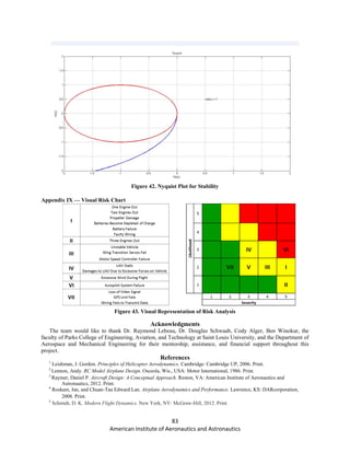

This document is a senior design report for an observational tilt-rotor unmanned aerial system called Paparazzi. The report describes the design of the Paparazzi UAS, which combines the capabilities of fixed-wing aircraft and rotorcraft to take off and land vertically while also efficiently cruising long distances. Key aspects of the design include a 40 inch wingspan, 5.5 pound weight, ability to hover for 15 minutes and cruise 4 nautical miles at 40 knots. The report details the conceptual design process, mission profile, weight breakdown, and aerodynamic analysis performed to develop the Paparazzi UAS for applications such as military reconnaissance, search and rescue, and commercial delivery.


