Other RLC resonant circuits and Bode Plots 2024

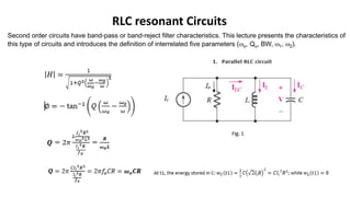
1. RLC resonant Circuits
Second order circuits have band-pass or band-reject filter characteristics. This lecture presents the characteristics of
this type of circuits and introduces the definition of interrelated five parameters (o, Qo, BW, 1, 2).

2. Example 1:
(a) A parallel resonant circuit with fo=800kHz. Assuming the input signal has an amplitude of 1, determine H at
850kHz Q=100. Also determine BW
Sol.
𝐻 =
1
1 + 𝑄2 𝜔
𝜔𝑜
−
𝜔𝑜
𝜔
2
=
1
1 + 1002 850
800
−
800
850
2
= 0.0832
∅ = − tan−1
𝑄
850
800
−
800
850
= −85.3°
𝐵𝑊 =
𝜔𝑜
𝑄
= 160𝜋
𝑟𝑎𝑑
𝑠𝑒𝑐
= 80𝐻𝑧

3. Practice:
1-A parallel RLC with 8k, 40mH, and 0.25sec. determine:
 Q,
 BW
 The cutoff frequencies.
2-A high-frequency parallel RLC resonant circuit has o of 10MRad/sec and BW =200kRad/sec. Determine Q and L if
C=10pF.
Summary of the definitions of Q:
 Q is the ratio of the inductor (and capacitor) current amplitude to the source current amplitude at resonance.
 Q is 2 times the ratio of the energy stored to the energy dissipated at the resonant state.
 Q is the ratio of the resonant frequency to the bandwidth.

5. Other RLC resonant circuits and Bode Plots
The first part of this lecture focuses of on deriving the filter parameters for any circuit focusing on internal
resistance and the effect of loading.
1. Including the effect of stray resistance
Practically energy storage components (inductors and capacitors) are not ideal as the elements models suggest. The
inductor, for instance, has resistance associated with its wire. The capacitor has stray wire resistance and dielectric leakage
conductance. Accordingly, idealized model –as studied in the last lecture- may cause significant error. Including stray and
shunt resistors spoils the simple parallel and series RLC configurations studied earlier. This section studies the resonant state
of any combination of second order RLC circuits focusing on the effect of non-ideal elements.
In this section we are going to consider –as common example- the effect of the inductor internal resistance on the parallel
RLC circuits, as shown in Fig. 1. For this circuit we are going to derive the filter parameters using two methods as follows.
C R
L
rL
Ii
Vo
Fig. 1

6. The direct method
The direct method depends on the definition of the resonant state as the state at which the transfer function (H(j)) is real
number (at resonance the imaginary part =0).
For the circuit shown in Fig. 1:
𝐻 𝑗𝜔 =
𝑉
𝑜
𝐼𝑜
= 𝑍𝑒𝑞
𝑍𝑒𝑞 =
1
𝑌𝑒𝑞
𝑌𝑒𝑞 =
1
𝑅
+
1
𝑟𝐿 + 𝑗𝜔𝐿
+ 𝑗𝜔𝐶
𝑌𝑒𝑞 =
𝑟𝐿 + 𝑗𝜔𝐿 + 𝑅 + 𝑗𝜔𝐶𝑅 𝑟𝐿 + 𝑗𝜔𝐿
𝑅 𝑟𝐿 + 𝑗𝜔𝐿
𝑌𝑒𝑞 =
𝑟𝐿 + 𝑅 − 𝜔2𝑅𝐿𝐶 + 𝑗𝜔 𝐿 + 𝐶𝑅𝑟𝐿
𝑅𝑟𝐿 + 𝑗𝑅𝜔𝐿
𝑍𝑒𝑞
=
𝑅𝑟𝐿 + 𝑗𝑅𝜔𝐿
𝑟𝐿 + 𝑅 − 𝜔2𝑅𝐿𝐶 + 𝑗𝜔 𝐿 + 𝐶𝑅𝑟𝐿
×
𝑟𝐿 + 𝑅 − 𝜔2𝑅𝐿𝐶 − 𝑗𝜔 𝐿 + 𝐶𝑅𝑟𝐿
𝑟𝐿 + 𝑅 − 𝜔2𝑅𝐿𝐶 − 𝑗𝜔 𝐿 + 𝐶𝑅𝑟𝐿

7. 𝑍𝑒𝑞
=
𝑅𝑟𝐿 𝑟𝐿 + 𝑅 − 𝜔2𝑅𝐿𝐶 + 𝑅𝜔2𝐿 𝐿 + 𝐶𝑅𝑟𝐿 + 𝑗 𝑅𝜔𝑟𝐿 𝑟𝐿 + 𝑅 − 𝜔2𝑅𝐿𝐶 − 𝑗𝑅𝑟𝐿𝜔 𝐿 + 𝐶𝑅𝑟𝐿
𝑟𝐿 + 𝑅 − 𝜔2𝑅𝐿𝐶 2 + 𝜔𝐿 + 𝜔𝐶𝑅𝑟𝐿
2
The imaginary part of 𝑍𝑒𝑞 = 𝑋𝑒𝑞
𝑋𝑒𝑞 =
−𝑅𝑟𝐿𝜔 𝐿 + 𝐶𝑅𝑟𝐿 + 𝑅𝜔𝐿 𝑟𝐿 + 𝑅 − 𝜔2𝑅𝐿𝐶
𝑟𝐿 + 𝑅 − 𝜔2𝑅𝐿𝐶 2 + 𝜔2 𝐿 + 𝐶𝑅𝑟𝐿
2
At resonance 𝑋𝑒𝑞 = 0
−𝑅𝑟𝐿𝜔𝑜 𝐿 + 𝐶𝑅𝑟𝐿 + 𝑅𝜔𝑜𝐿 𝑟𝐿 + 𝑅 − 𝜔𝑜
2
𝑅𝐿𝐶 = 0
−𝑟𝐿𝐿 − 𝐶𝑅𝑟𝐿
2 + 𝐿𝑟𝐿 + 𝐿𝑅 − 𝜔𝑜
2𝑅𝐿2𝐶 = 0
𝜔𝑜
2
𝑅𝐿2
𝐶 = 𝐿𝑅 − 𝐶𝑅𝑟𝐿
2
𝜔𝑜
2𝐿2𝐶 = 𝐿 − 𝐶𝑟𝐿
2
𝜔𝑜
2 =
𝐿 + 𝐶𝑟𝐿
2
𝐿2𝐶
=
1
𝐿𝐶
−
𝑟𝐿
2
𝐿2
𝝎𝒐 =
𝟏
𝑳𝑪
−
𝒓𝑳
𝟐
𝑳𝟐

8. At this point, if we want to carry on the analysis to find other parameters using symbolic parameters, we will face tedious
analytical manipulations. This process can be mitigated if we use numerical –rather than symbolic- parameters. Example 1
shows complete analysis.
Example 1: Determine the following parameters of the circuit shown in Fig. 2: 𝜔𝑜, 𝑄, 𝐵𝑊, 𝜔𝑐1, 𝜔𝑐2
Fig. 2
Sol.
From the analysis above
𝜔𝑜 =
1
𝐿𝐶
−
𝑟𝐿
2
𝐿2
=
1
5 × 10−10
−
64
25 × 10−8
= 41,761 𝑟𝑎𝑑/𝑠𝑒𝑐
To determine Q:
 Determine H(o),
 Determine the Energy stored and Energy Dissipated at resonance.
 Find Q

9. 𝐻 𝜔𝑜 =
1
𝑗𝜔𝑜𝐶
𝑅𝑙 + 𝑗𝜔𝑜𝐿 𝑅𝑠
We substitute the numerical values of the components and o
𝐻 𝜔𝑜 = 55.56∠0°
𝑉
𝑜 𝜔 = 𝜔𝑜 = 𝐼𝑖 × 𝐻 𝜔𝑜 = 0.04 × 55.56∠0°
𝑉
𝑜 𝜔 = 𝜔𝑜 = 2.22∠0°𝑉
The current in the L branch:
𝐼𝐿 𝜔 = 𝜔𝑜 =
2.22∠0°
8 + 𝑗0.5𝑚 × 41761
≅ 0.1∠ − 69°𝐴
The energy dissipated in Rs
𝑊𝑅𝑠 =
𝑉
𝑜
2
𝑅𝑠
1
𝑓0
=
2.222
500
2𝜋
41 761
= 1.4859𝜇𝐽
𝑊𝑅𝑙 = 𝐼𝐿
2
𝑅𝑙
1
𝑓0
= 0.01 × 8 ×
2𝜋
41 761
= 12.036𝜇𝐽
To Determine the energy stored assume (the arbitrary angle of the supply current=0), or:
𝑖𝑠 = 40 2cos(41761𝑡)
Gives 𝑣𝑜 𝑡 = 0 = 3.14𝑉

10. The energy stored in the capacitor at (t=0) is:
𝑤𝑐 𝑡 = 0 =
1
2
× 10−6 × 3.142 = 4.9298𝜇𝐽
at t=0, the current in the inductor;
𝑖𝐿 𝑡 = 0 = 0.1 2 cos −69 = 0.0507𝐴
The corresponding inductor current:
𝑤𝐿 𝑡 = 0 =
1
2
× 0.5 × 10−3
× (0.0507)2
= 0.642𝜇𝐽
𝑄 = 2𝜋
𝑤𝐿 + 𝑤𝐶
𝑤𝑅𝑠 + 𝑤𝑅𝑙
= 2𝜋
5.5718
13.52
=
𝐵𝑊 =
𝜔𝑜
𝑄
=
41761
2.59
= 16,132𝑟𝑎𝑑/𝑠𝑒𝑐
The cutoff frequencies:
𝜔1 = 41761 1 +
1
2.59
2
−
16132
2
= 36700𝑟𝑎𝑑/𝑠𝑒𝑐
𝜔1 = 41761 1 +
1
2.59
2
+
16132
2
= 52830𝑟𝑎𝑑/𝑠𝑒𝑐

11. Equivalent-circuit method
As an alternative method for analysis, we are going to replace the series 𝑟𝐿𝐿 branch with the equivalent parallel
resistance and inductance as explained in Fig. 3. After that the circuit of Fig. 1 becomes a pure parallel RLC resonant circuit.
L
rL
Lp
rp
Fig. 3
The series branch impedance is:
𝑍 = 𝑟𝐿 + 𝑗𝜔𝐿
And the equivalent admittance:
𝑌 =
1
𝑟𝐿 + 𝑗𝜔𝐿
=.
𝑟𝐿 − 𝑗𝜔𝐿
𝑟𝐿
2 + 𝜔𝐿 2
𝑌 =
1
𝑟𝑝
+
1
𝑗𝜔𝐿𝑝

12. Gives:
𝑟𝑝 =
𝑟𝐿
2+ 𝜔𝐿 2
𝑟𝐿
And 𝜔𝐿𝑝 =
𝑟𝐿
2+ 𝜔𝐿 2
𝜔𝐿
𝐿𝑝 =
𝑟𝐿
2
+ 𝜔𝐿 2
𝜔2𝐿
The resonant frequency of the circuit shown in Fig. 4 (which is the circuit configuration after replacing the series branch by its parallel equivalent) satisfies the
equation:
𝜔𝑜
2
=
1
𝐿𝑝𝐶
=
𝜔𝑜
2𝐿
𝐶𝑟𝐿
2
+ 𝐶𝜔𝑜
2𝐿2
𝜔𝑜
2
𝐶𝑟𝐿
2
+ 𝐶𝜔𝑜
4𝐿2 = 𝜔𝑜
2𝐿
Divide by 𝜔𝑜
2
𝐶𝑟𝐿
2
+ 𝐶𝜔𝑜
2
𝐿2
= 𝐿
𝐶𝜔𝑜
2
𝐿2
= 𝐿 − 𝐶𝑟𝐿
2
𝜔𝑜
2
=
𝐿 − 𝐶𝑟𝐿
2
𝐶𝐿2
=
1
𝐿𝐶
−
𝑟𝐿
2
𝐿2
𝜔𝑜 =
1
𝐿𝐶
−
𝑟𝐿
2
𝐿2
𝑄 = 𝑅𝑒𝑞𝜔𝑜𝐶
Where 𝑅𝑒𝑞 = 𝑟𝑝𝑅
C R
L
rL
Ii
Vo
C R
Ii
Vo
Lp
rp

13. 2-Cascaded Filters
Many electronic systems are arranged as cascaded stages as shown in Fig. 5.
H1(j) H2(j) H3(j)
V1 V2 V3 V4
If we assume that the transfer functions are not affected by loading, the transfer function of the cascaded system:
H(jω)=V4V1=V2V1×V3V2×V4V3=H1×H2×H3
Fig. 5

14. 3- Bode Plots
Bode plot is a tool used to draw the variation of the transfer function (H) with the frequency. Bode diagram
has two graphs drawn on the same frequency scale; (i) |H(j)| and (j) therefore it is also known as the
gain and phase plot. Bode Plot is drawn using a semi-log graph paper as shown in Fig. 6.
One Decade
Fig. 6
The base-10 log axis is used as a frequency axis. The cycle of
the frequency axis is called a decade. The graph paper shown in
Fig. 6 has 4 decades therefore its maximum frequency is 104
the minimum frequency.
The amplitude of transfer function (A) in Bode plots is draws
using logarithmic unit know as dB (for decibel or deci-Bell),
where:
𝐴 𝑖𝑛 𝑑𝐵 = 20 log( 𝐻 )
In this section we will show how to draw the Bode diagram of a
LPF and HPF.