electronics

1. Important points to remember before starting the lecture
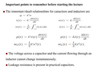
■ The important (dual) relationships for capacitors and inductors are
■ The voltage across a capacitor and the current flowing through an
inductor cannot change instantaneously.
■ Leakage resistance is present in practical capacitors.

2. ■ When capacitors are interconnected, their equivalent capacitance
is determined as follows: capacitors in series combine like resistors
in parallel, and capacitors in
parallel combine like resistors in series.
>> In dc steady state, a capacitor looks like an open circuit and an
inductor looks like a short circuit.
■ When inductors are interconnected, their equivalent inductance is
determined as follows: inductors in series combine like resistors in
series, and inductors in parallel combine like resistors in parallel.

3. Topic 7.1
First Order Differential circuits:
Those Circuits that contain only a single storage element e.g.
Capacitor or Inductor. The network can be describe as first-order differential
equation.
Analysis:
It involves an examination and description of behavior of a circuit
as a function of time after a specific change occurs in the network due to
switches opening and closing.
Time Constant (τ):
The time taken by an electrical circuit to charge the storing element.
For conductor (τ)=L/R
For Capacitor (τ)= RC

4. Topic 7.2
First-Order differential derivation
Consider a first-order differential equation of the from
A fundamental theorem of differential equation states that if
X(t) = X p (t) is any solution to Eq.(7.1) and x(t) = X c (t) is any
solution of homogeneous equation
then
The term X p (t) is called the particular integral solution, or
forced response, and X c (t) is called the complementary
solution ,or natural response the situation in which f(t) = A
( ) ( ) 7.1
dx
t ax f t
dt
 
( ) 0 7.2
dx
t ax
dt
 
( ) ( ) ( ) 7.3
p c
x t x t x t
 
( ) 7.4
P
P
dx
t ax A
dt
 

5. since the right –hand side of Eq . (7.3) is a constant,
it is reasonable to assume that the solution X p (t) must also be a
constant therefore, we assume that
X p (t) = K 1
Substituting this constant into Eq.(7.4) yields
K 1 =A / a
Examining Eq.(7.5) we note that
the equation is equivalent to
therefore ,
( ) ( ) 0 7.5
C
C
dx
t ax t
dt
 
( ) / ( ) 7.6
C
C
dx
t x t a
dt
 
 
 
 
[ln ( )] 7.7
ln ( ) 7.8
C
C
d
x t a
dt
x t at C
 
 
 
 
  
2
( ) 7.9
at
C
x t k e


6. 1 2
1 2
1
2
( ) ( ) ( )
, ( )
1
, ( )
steady-state solution:
( )
p c
at
t
t
we knowthat
x t x t x t
so x t k k e
as a
so x t k k e
where k
A
x t k e
a






 
 

 

 

8. ( ) ( )
0
( ) ( )
0
( ) ( )
0
( ) ( )
dv t v t vs
C
dt R
dv t v t Vs
C
dt R R
dv t v t Vs
dt CR CR
dv t v t Vs
dt CR CR

 
  
  
 
First-Order circuits electrical network derivation: state-variable approach.
Consider the circuit shown, At time the switch closes. The KCL equation that
describes the capacitor voltage for time is

9. /
1 2
/ /
1 2 1 2
/ /
2 1 2
/ /
1 2
2
/ /
1 2
2
/ /
2 1 2
( )
( )
1
1
1
( )
1
(
t
t t
t t
t t
t t
t t
v t k k e
d k k e k k e Vs
dt CR CR
k k k Vs
e e
dt CR CR CR
k k Vs
k e e
CR CR CR
We knowthat CR
k k Vs
k e e
CR CR CR CR
Taking CR common
Vs
k e k k e
CR CR
CR

 
 
 
 
 



 
 
 
 
 
 
 
 
   
   

   
   
1 1
) ,
Vs Vs
k k CR
CR CR
 
we assume that the solution of this first-order differential equation is of the form

10. Hence, the complete solution for the voltage v(t) is
1
/
1 2
/
2
( )
( )
t
t
k vs
RC
we Knowthat
v t k k e
v t vs k e







 
 
Where V is the steady-state value and RC is the network’s time
constant. K2 is determined by the initial condition of the capacitor. For
example, if the capacitor is initially uncharged (that is, the voltage
across the capacitor is zero at t=0 ), then
So, we obtain

11. Example 7.1: Consider the circuit shown. Assuming the
switch has been in position 1 for a long time.
At time t=0 the switch is moved to position 2.
At t=0- the capacitor is fully charged and conducts no current
since the capacitor acts like an open circuit to dc.
  2
2
0 arg
3
0 12 4
1 6 3
s
at t capacitor is fully ch ed
R K
Vc V v
R R K K


 
 
 
  
 

12.      
 
 
 
 
 
 
1 2
1 2
0
1
0
1
&
1
0
6 3
5
1
0
1 1
dv t V t v t
C
dt R R
dv t
C V t
dt R R
Dividivg throgh out by putting the
C
component values we get
dv t
V t
dt C
dv t
v t
dt
  
  

 
 
 
 





 

The network for t > 0 the KCL equation for the voltage across the
capacitor is

13.  
 
   
 
/
2
/.2
2
0.2sec ,
0 0 4 ,
4
t
t V
The form of the solution to this
homogeneous equation is
V t K e
If we substitute this solution into
the differential equation
thus
V t K e
Using the initial condition
Vc Vc V
V t e







   

   
 
/.2
2
/.2
/
4 / 3
t V
t mA
I t V t R
I t e





14. Example 7.2: The switch in the network in Fig. 7.5a opens at t=0. Let
us find the output voltage V0(t) for t>0
At t = 0- the circuit is in steady state and the inductor acts like a
short circuit.
The initial current through the inductor can be found in many
ways;
however, we will form a Thevenin equivalent for the part of the
network to the left of the inductor, as shown in fig.

15. The network for t > 0 shown. Note that the 4-V independent
source and the 2-ohm resistor in series with it no longer have
any impact on the resulting circuit.
Vnet=4+12=16
1 2
1
1 2
1 2
1
2 2 4
16
4
4
2 2
1
2 2
4 1 4
&
t
eq
net
eq
th
t
h th
h h
t
Now we fi
R R R
V
I A
R
R R
R
R R
n
I R V
d V R
V
     
  
 
   
 
   


16.  
 
1
/
1 2
/
1 2
/
1 2
/ /
2 2
2(0)
2
2
2
(0 )
3
.5
( )
0
2 6
1
6 2 0 6
1.33 3
1.33 3
3 1.33
L
t
t
t
t t
Now find i
K
i t K K e
Now for t KVL equation
d K K e
K K e V
dt
K e K e V
K e
K
K



 






 



 


  

 
   
 
 
 
 
 

17. 2
1 3 1
1 3
(0 )
1 2 3
4
1.33
3
0
( )
( ) ( )
( )
( ) ( ) 2 12
L
NET th
th
L
NET
S
Now find i
R R R
V
i A
R
Now for t KVL equation
di t
R i t L R i t V
dt
di t
R R i t V
dt

     
  

  
  

18. 1
1
/
2
/0.5 2
1 2 2
2
2
2,
2 2 ( )
( ) 6
2
( )
2 ( ) 6
0 2 ( ) ( )
2 ( ) 6 ( ) 3
( )
( )
2
0.5sec
4
( ) 3
1.33 3
P
t
c
eq
t t
t
Dividing Through out with
di t
i t V
dt
di t
i t V
dt
At t i t X t K
i t V i t V K
di t
X t K e
dt
L
R
i t K K e K e
K e
Students solv further



 


 
 
   
   
  
  
   
 

19. Applying Differential Method Step-by-Step to solve The Problems:

21.  
Consider the circuit. The circuit is in steady state
prior to time t=0,when the switch is closed.
Let us calculate the current i(t) for
1. 0 ?
,
Solution
Example 7.3
 


Step i t at t
Let  
 
1 2
2. 0 ?
36 12 24
2 6 4 12


 
 
  
       
t
c
net
net
Step
i t k k e
v
v v v v
R k k k k
t > 0

22.  
 
 
1
24
2
12
2 2 4
0 36 4 32
0
3.
R
c
v
i t mA
k
v IR
mA k V
v v v v
i t at t
Step

 


   
   

   
 
 
1 2
0
32 16
6 3
0
36 36 36 9
2 6 8 2
4.
c
v
i t
R
v
mA
k
i t at t
v v v
i mA
R R k k k
Step


 


    
   

23.   
     
 
3 6
1
2 6 12 3
2 6 8 2
3
10 100 10 0.15
2
9
2
5.
,
6.
TH
TH
k k k
R k
k k k
R C
s
k i mA
k
Step
Therefore
Step


  
   
  

 
  
   
 
2
0.15
0
16 9 5
3 2 6
9 5
2 6
,
t
s
i i
mA mA mA
i t e mA
Hence

   
  
 

24. 0.
( ) 0
1.
Example 7.4
The circuit is assumed to have been in a steady state
condition prior to switch closure at t
We wish to calculate the voltage v t for t
Step
Solution




 
    
1 2
.
24 6
0
6 3 6 3
4
6 3
24 8
6
6 3
9
2
t
L
v t k k e
v
i
v
A
Step


 
 

   
    
 

  
 

 
 
 
 
 

25.  
   
 
     
 
1
1 1 1
0
8
0 0
3
0 ?
0 24 0 0
8
0
4 6 3 12
3 0 72 2
1
3.
L
L L
i t at t
i i A
v
v v v v
A
v
Step
 
   
 
   
   
  
      
 
 
 
1
1
1
0 32 0
1 1 0
12
6 0 40 = 0
6 0 = 40
40 20
0 = =
6 3
v v
v
v
v v
   

 



26.    
1
20
0 24 0 24
3
72 20 52
3 3
( )
6, 12, 1, 2 ,
,
4.
,
v v v v v
v
I
v
f and resistors are shorted
Then
Step
Therefore
     

 


24
4, 6, 12 .
1 1 1 1 3 2 1 6
4 6 12 12 12
12
2
6
5.
,
TH
TH
TH
V
R is equal to the and resistors in parallel
R
R
Step
Then


 
    
  

27.  
   
1
2
4
2
2
24
0
52 52 72 20
24
3 3 3
,
6.
,
TH
L
s
R
k v v
k v v
Then
Step
Hence
   
  
   

    
  2
20
24
3
t
s
v t e v

 

28. Topic 7.3:
Second order-circuits: Let us consider basic RLC circuit.
Assume energy is stored(already charged) in both inductor and
capacitor parallel RLC circuit is
   
 
0
2
2
( )
CKT
1
Multiplying by we get
+0+
L s
s
The node equation of the given RLC parallel
V dv
V dt I t C I t
R L dt
d
dt
di t
d V V d
t
v
C
dt R L dt dt
   

 


29. 2
1 2
2
2
1 2
2
, , tan ,
a ( )
hom
a 0
Heretaking R L C cons t
In general we can write differential equation as
d v dV V
a f t
dt dt L
From above we can write ogeneous equation as
d v dV V
a
dt dt L
  
  
Here we apply the same approach as in Ist order CKTs that is
x(t)=xp(t) and x(t)=xc(t)
Hence x(t) = xp(t) + xc(t)
We put f(t)=A such that x(t) = A/a2+ xc(t)
Let us now turn our attention to the solution of the homogeneous
equation 2
2
0 0
2
2 0
d v dV V
dt dt L
 
  
is called the exponential damping ratio, and ω0 is referred to as the
undamped natural frequency.
𝜍

30. 2 2
0
st
st s t
0
t s
st
2
2
Again we assume that
x(t) = Ke
Substituting this expression into hom
Ke Ke Ke
Dividing both sides of the equation
0
2
by Ke gives
ogenious
equation and converting to frequency domain gives
s s
s
 

  
 2
0 0
This equation is commonly called the
characteristic equatio
0
n;
s
 
 
Employing the quadratic formula, we find

31. Such That
In general, then, the complementary solution of homogeneous
eq. is

32. Example # 7.9
Q. Use the differential equation approach to find Vo(t) for t > 0 in Circuit and plot the
response including the time interval just prior opening the switch.
Here Vc (0+) = Vc (0-) = R2 / R2 + R3 x 12= 6v
Now for t > 0:
Vo = - R3 / R1 + R3 x Vc = - x Vc (1)
Here x = R3 / R1 + R3 ,
And Vc / R2 + c dVc / dt = Vo / R3 (2)
From eq. 1 & 2
dVo / dt + Vo [ 1 / R2c + x / R3c ] = 0 (3)
Let the sol. of above eq. 3
Vo (t) = k e^-t/c
Here c = 1 / 1/ R2c + x / R3c = C R2 (R1 + R3) / R1 + R2 + R3
= 7200/ 18k = 0.4 p
And Vo (0+) = - Vc (0+).x = -6 x ½ = -3v
K = -3
So: Vo (t) = -3 e – t/0.4 v for t > 0

33. Example # 7.10
Q. In the network in fig. find io(t) for t > 0 using the differential equation approach.
Here iL (0-) = 2 x 1 / R1 / 1/ R1 + 1/ R2 + 1/ R3
= 2 x 1/6 x 288/ 144 = 0.66 A
At t = 0+
Io = IL = 0.66 A
Now for t > 0
L diL / dt + io (R1 + R2) = 0 and io = iL
dio / dt + R1 + R2 / L io = 0
dio / io = - R1 + R2 / L dt
Sol. Of the above equation:
Io = A e-t/c
C = L / R1+ R2 = 2/10 = 1/5
Io ( 0+) = k = 0.66 A
Because io (t) = 0.66 e^-5t A

34. Example # 7.11
Q. Use the differential equation approach to find IL(t) for t > 0 in the circuit and plot the
response , including the interval time interval just prior to opening the switch. Given ckt. for
t = - 0
Voltage chop across R3:
V = RB / RA + RB × 6 = 2 V
And IL (0-) = V/ R4 = 2/3 A
Now for t > 0 :
Applying KVL : L diL(t)/ dt +( R3 + R4 )IL(t)=0
DIL(t) / I L (t) = - R3+ R4 /L d t
Soluton of above eq.
IL (t) = A e^- (R3 +R4) t
= A e ^-4.5 t
Because IL (0-)=IL (0+)= 2/3 A = 2/3
So IL (t) = 2 / 3 e^-4.5 t