Download to read offline


![Datalog§ [Cali’ et Al, PODS 09]
¡ Datalog variant allowing in the head:
- 9-variables ! TGDs 8X8Y (X,Y) 9Z (X,Z)
- Equality atoms ! EGDs 8X (X) Xi=Xj Datalog+
- Constant false (?) ! NCs 8X (X) ?](https://image.slidesharecdn.com/orsivldb11-13154779239988-phpapp01-110908053319-phpapp01/75/Orsi-Vldb11-7-2048.jpg)
![Datalog§ [Cali’ et Al, PODS 09]
¡ Datalog variant allowing in the head:
- 9-variables ! TGDs 8X8Y (X,Y) 9Z (X,Z)
- Equality atoms ! EGDs 8X (X) Xi=Xj Datalog+
- Constant false (?) ! NCs 8X (X) ?
¡ But, query answering under Datalog+ is undecidable](https://image.slidesharecdn.com/orsivldb11-13154779239988-phpapp01-110908053319-phpapp01/75/Orsi-Vldb11-8-2048.jpg)
![Datalog§ [Cali’ et Al, PODS 09]
¡ Datalog variant allowing in the head:
- 9-variables ! TGDs 8X8Y (X,Y) 9Z (X,Z)
- Equality atoms ! EGDs 8X (X) Xi=Xj Datalog+
- Constant false (?) ! NCs 8X (X) ?
¡ But, query answering under Datalog+ is undecidable
¡ Datalog+ is syntactically restricted ! Datalog§](https://image.slidesharecdn.com/orsivldb11-13154779239988-phpapp01-110908053319-phpapp01/75/Orsi-Vldb11-9-2048.jpg)
![Datalog§ [Cali’ et Al, PODS 09]
¡ Datalog variant allowing in the head:
- 9-variables ! TGDs 8X8Y (X,Y) 9Z (X,Z)
- Equality atoms ! EGDs 8X (X) Xi=Xj Datalog+
- Constant false (?) ! NCs 8X (X) ?
¡ But, query answering under Datalog+ is undecidable
¡ Datalog+ is syntactically restricted ! Datalog§
¡ TGDs more expressive than inclusion dependencies
8D8P8A runs(D,P),area(P,A) 9E employee(E,D,A)](https://image.slidesharecdn.com/orsivldb11-13154779239988-phpapp01-110908053319-phpapp01/75/Orsi-Vldb11-10-2048.jpg)
![Query Answering via Chase
Q h
C = chase(D,)
D
h1 h2
h2(C)
h1(C) . . .
M1
M2
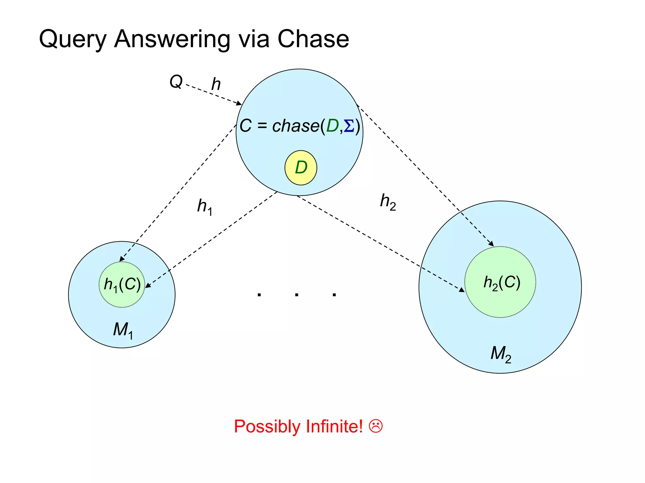
D[²Q , chase(D,) ² Q
[see, e.g., Deutsch, Nash & Remmel, PODS 08]](https://image.slidesharecdn.com/orsivldb11-13154779239988-phpapp01-110908053319-phpapp01/75/Orsi-Vldb11-16-2048.jpg)
![FO-rewritability: Example [Gottlob et Al., ICDE 11]
promoter(X) Y promotesTo(X,Y)
promotesTo(X,Y) customer(Y)
Q q promotesTo(A,B), customer(B)
Q
q promotesTo(A,B), customer(B) (original query)](https://image.slidesharecdn.com/orsivldb11-13154779239988-phpapp01-110908053319-phpapp01/75/Orsi-Vldb11-26-2048.jpg)
![FO-rewritability: Example [Gottlob et Al., ICDE 11]
promoter(X) Y promotesTo(X,Y)
promotesTo(X,Y) customer(Y)
Q q promotesTo(A,B), customer(B)
Q
q promotesTo(A,B), customer(B) {Y=B}
q promotesTo(A,B), customer(V0,B) ( V0 is fresh )](https://image.slidesharecdn.com/orsivldb11-13154779239988-phpapp01-110908053319-phpapp01/75/Orsi-Vldb11-27-2048.jpg)
![FO-rewritability: Example [Gottlob et Al., ICDE 11]
promoter(X) Y promotesTo(X,Y)
promotesTo(X,Y) customer(Y)
Q q promotesTo(A,B), customer(B)
Q
q promotesTo(A,B), customer(B)
factorization
q promotesTo(A,B), promotesTo(V0,B) ans(A) promotesTo(A,B)
{ A = V0 }](https://image.slidesharecdn.com/orsivldb11-13154779239988-phpapp01-110908053319-phpapp01/75/Orsi-Vldb11-28-2048.jpg)
![FO-rewritability: Example [Gottlob et Al., ICDE 11]
promoter(X) Y promotesTo(X,Y)
promotesTo(X,Y) customer(Y)
Q q promotesTo(A,B), customer(B)
Q
q promotesTo(A,B), customer(B)
q promotesTo(A,B) {X = A, Y = B}
q promoter(A)](https://image.slidesharecdn.com/orsivldb11-13154779239988-phpapp01-110908053319-phpapp01/75/Orsi-Vldb11-29-2048.jpg)
![FO-rewritability: Example [Gottlob et Al., ICDE 11]
promoter(X) Y promotesTo(X,Y)
promotesTo(X,Y) customer(Y)
Q q promotesTo(A,B), customer(B)
Q
q promotesTo(A,B), customer(B)
q promotesTo(A,B) UCQ rewriting
(first-order)
q promoter(A)](https://image.slidesharecdn.com/orsivldb11-13154779239988-phpapp01-110908053319-phpapp01/75/Orsi-Vldb11-30-2048.jpg)

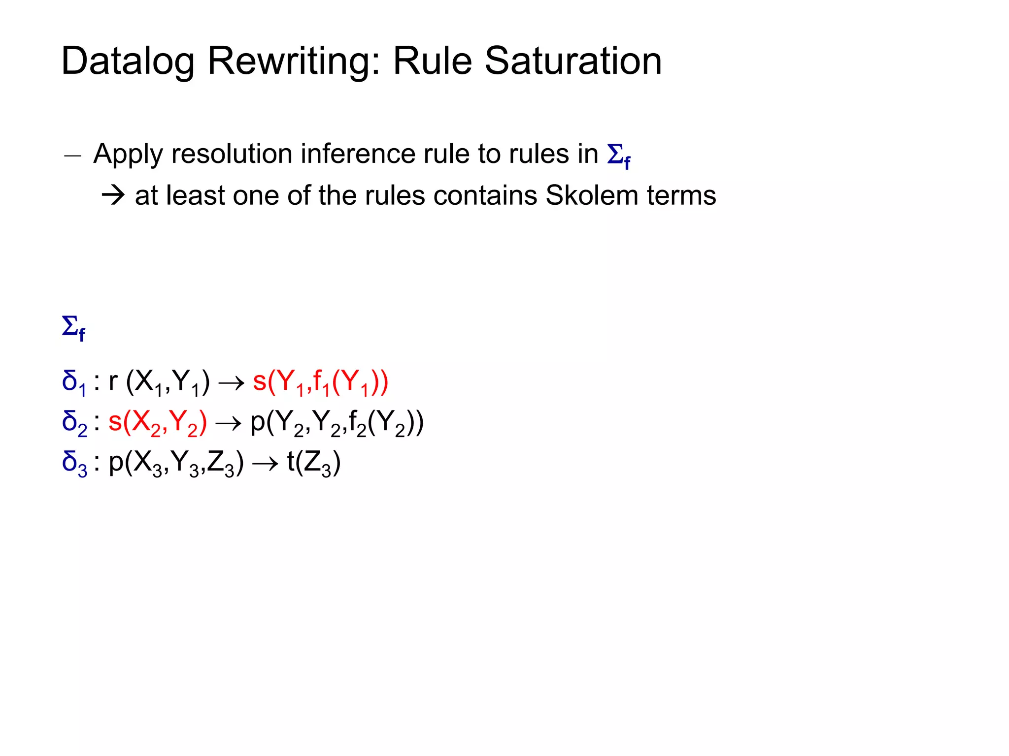
![Datalog Rewriting: Rule Saturation
¡ Apply resolution inference rule to rules in f
at least one of the rules contains Skolem terms
f [f]
δ1 : r (X1,Y1) s(Y1,f1(Y1)) …
δ2 : s(X2,Y2) p(Y2,Y2,f2(Y2)) r(X1,Y1) p(f1(Y1) ,f1(Y1), f2(f1(Y1)))
δ3 : p(X3,Y3,Z3) t(Z3) …](https://image.slidesharecdn.com/orsivldb11-13154779239988-phpapp01-110908053319-phpapp01/75/Orsi-Vldb11-53-2048.jpg)
![Datalog Rewriting: Properties of Rule Saturation
¡ [f] mimics the chase derivations.](https://image.slidesharecdn.com/orsivldb11-13154779239988-phpapp01-110908053319-phpapp01/75/Orsi-Vldb11-54-2048.jpg)
![Datalog Rewriting: Properties of Rule Saturation
¡ [f] mimics the chase derivations.
δ1 : r (X1,Y1) s(Y1,f1(Y1))
δ2 : s(X2,Y2) p(Y2,Y2,f2(Y2))
δ3 : p(X3,Y3,Z3) t(Z3)](https://image.slidesharecdn.com/orsivldb11-13154779239988-phpapp01-110908053319-phpapp01/75/Orsi-Vldb11-55-2048.jpg)
![Datalog Rewriting: Properties of Rule Saturation
¡ [f] mimics the chase derivations.
δ1 : r (X1,Y1) s(Y1,f1(Y1))
δ2 : s(X2,Y2) p(Y2,Y2,f2(Y2))
δ3 : p(X3,Y3,Z3) t(Z3)
¡ [f] depends only on .
¡ [f] is possibly infinite
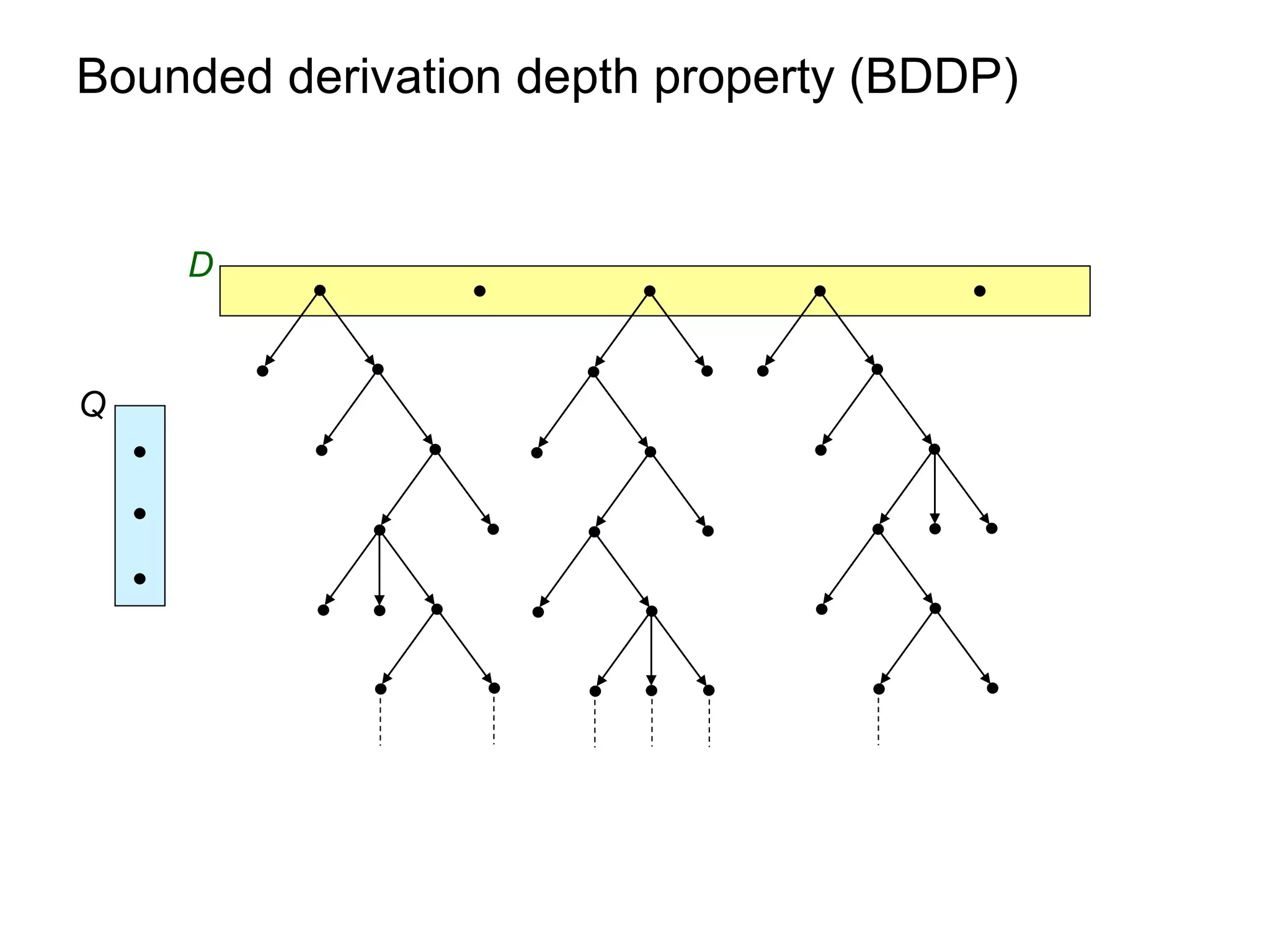
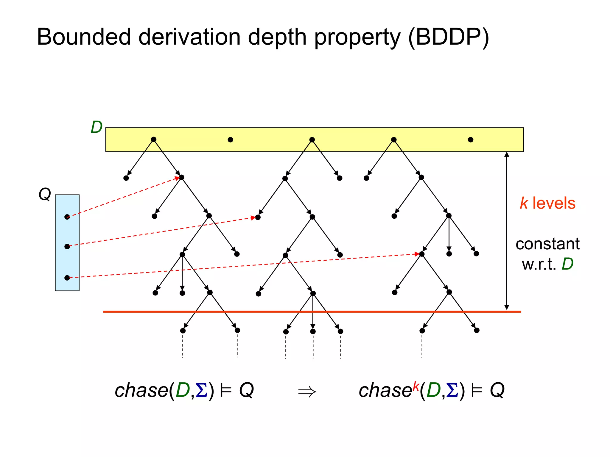
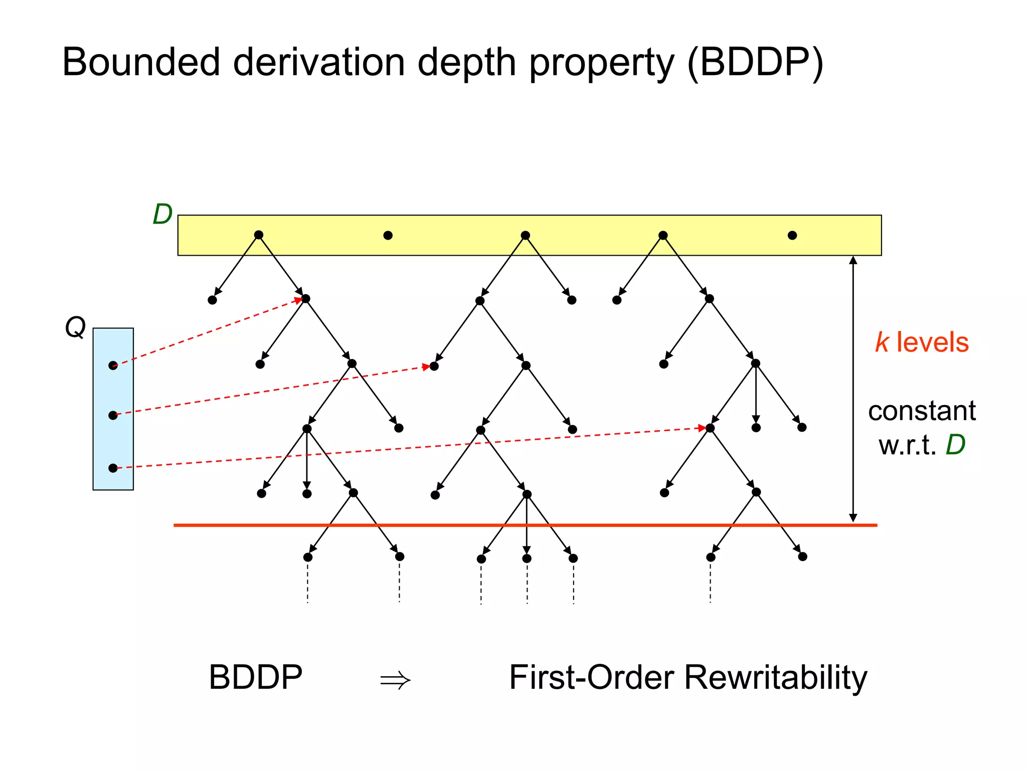
linear TGDs have BDDP: suffices to construct it up to k steps [f]k.](https://image.slidesharecdn.com/orsivldb11-13154779239988-phpapp01-110908053319-phpapp01/75/Orsi-Vldb11-56-2048.jpg)
![Datalog Rewriting: Query Saturation
¡ resolve [f] with the query Q.
use only rules with Skolem terms.](https://image.slidesharecdn.com/orsivldb11-13154779239988-phpapp01-110908053319-phpapp01/75/Orsi-Vldb11-57-2048.jpg)
![Datalog Rewriting: Query Saturation
¡ resolve [f] with the query Q.
use only rules with Skolem terms.
[f] … Q
Q s(A,B), p(B,B,C)
δ1 : r (X1,Y1) s(Y1,f1(Y1))
δ2 : s(X2,Y2) p(Y2,Y2,f2(Y2))
δ3 : p(X3,Y3,Z3) t(Z3)
…
[δ12]] : r (X1,Y1) p(f1(Y1) ,f1(Y1), f2(f1(Y1)))
…
…
[Q,f] Q r(X1,Y1), p(f1(Y1), f1(Y1),C)
…](https://image.slidesharecdn.com/orsivldb11-13154779239988-phpapp01-110908053319-phpapp01/75/Orsi-Vldb11-58-2048.jpg)
![Datalog Rewriting: Query Saturation
¡ bypasses chase derivations with function symbols
Q
Q s(A,B), p(B,B,C)
[f] …
δ1 : r (X1,Y1) s(Y1,f1(Y1))
δ2 : s(X2,Y2) p(Y2,Y2,f2(Y2))
δ3 : p(X3,Y3,Z3) t(Z3)
…
[δ12]] : r (X1,Y1) p(f1(Y1) ,f1(Y1), f2(f1(Y1)))
…](https://image.slidesharecdn.com/orsivldb11-13154779239988-phpapp01-110908053319-phpapp01/75/Orsi-Vldb11-59-2048.jpg)
![Datalog Rewriting: Finalization
¡ keep only the function-free rules from [f] [ [Q,f]
¡ derivations producing certain answers are captured by function-
symbol-free rules.
¡ (optional) add auxiliary rules to make the rewriting a proper Datalog
query i.e., clear distinction IDB/EDB.](https://image.slidesharecdn.com/orsivldb11-13154779239988-phpapp01-110908053319-phpapp01/75/Orsi-Vldb11-60-2048.jpg)
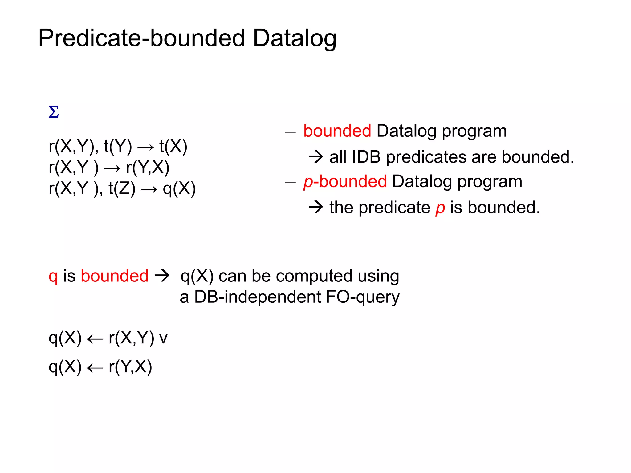
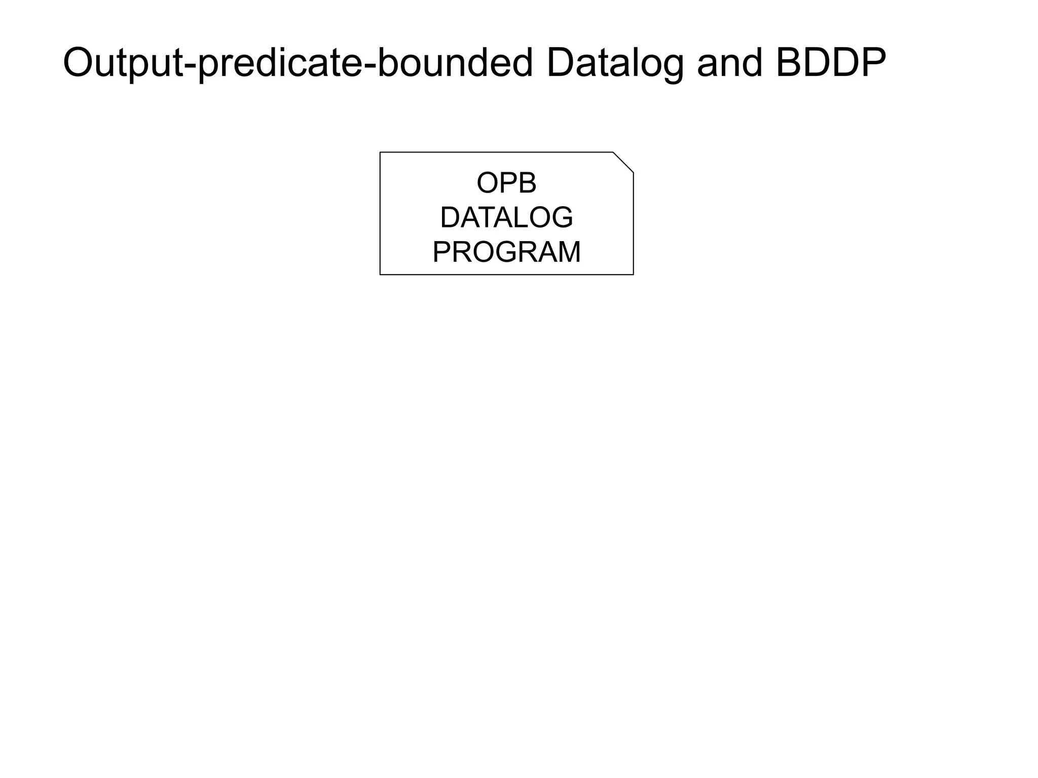
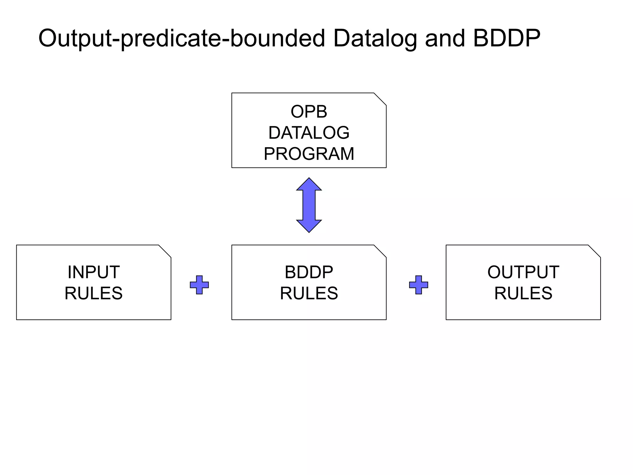
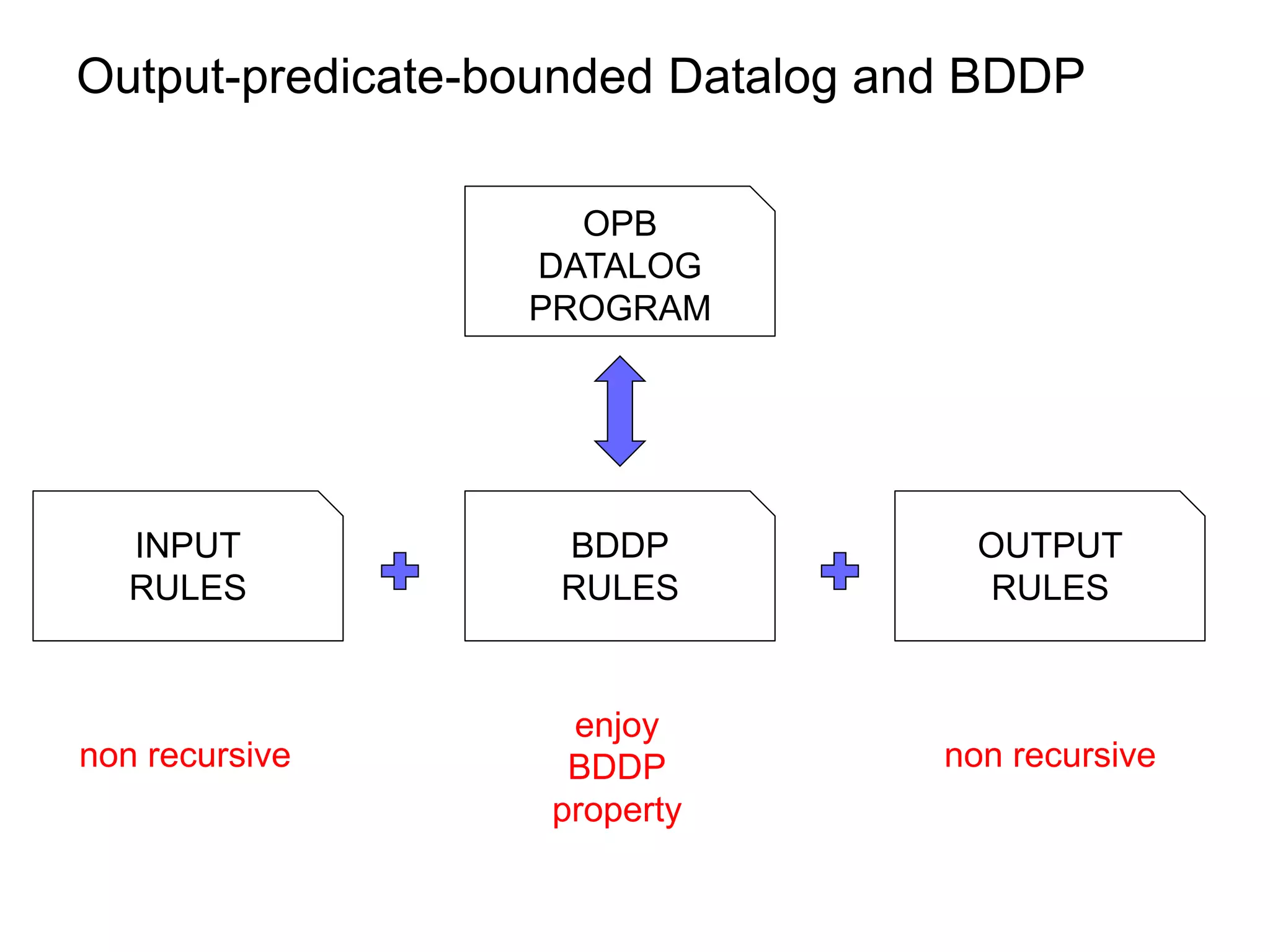
![OPB-Datalog and BDDP revisited
OPB
DATALOG
PROGRAM
INPUT BDDP OUTPUT
RULES RULES RULES
aux ff([f]) ff([Q,f])
enjoy
non recursive BDDP non recursive
property](https://image.slidesharecdn.com/orsivldb11-13154779239988-phpapp01-110908053319-phpapp01/75/Orsi-Vldb11-61-2048.jpg)
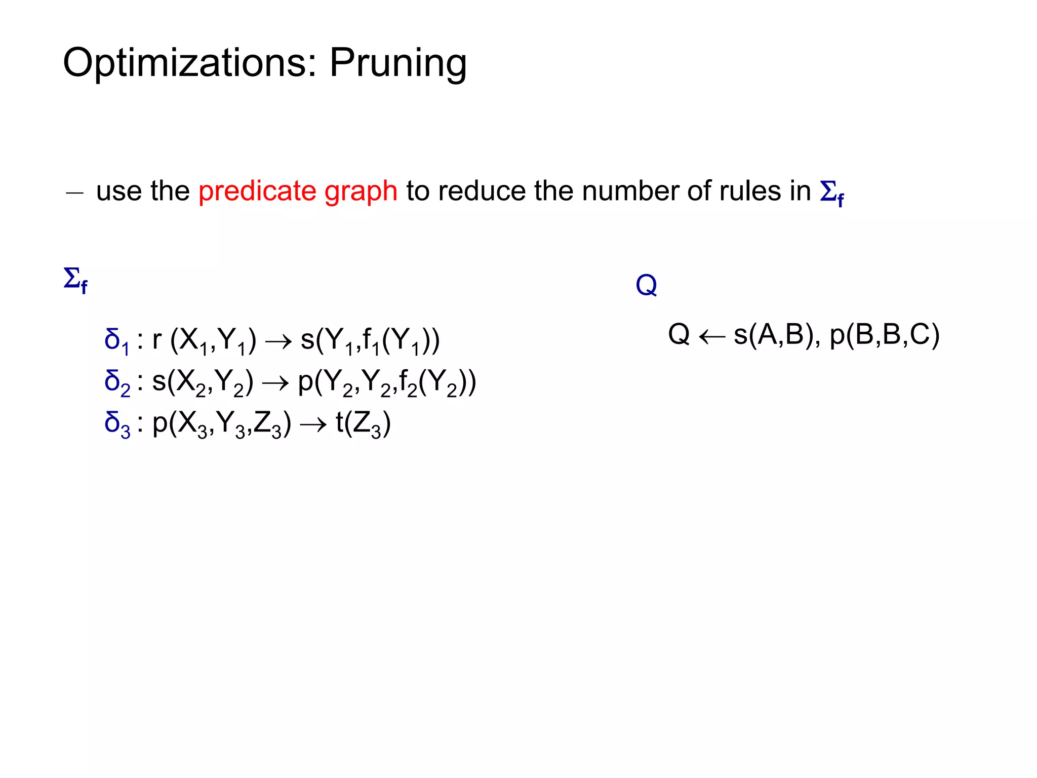
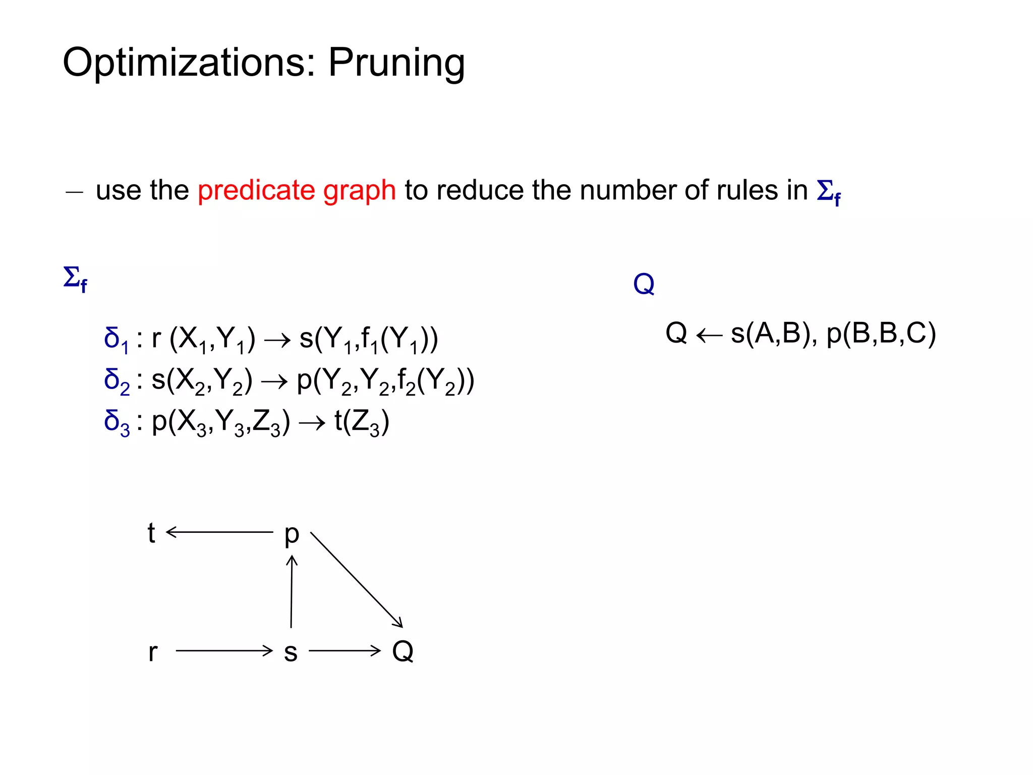
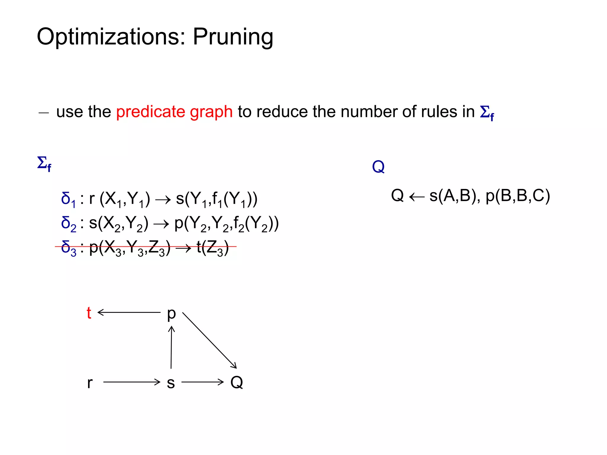
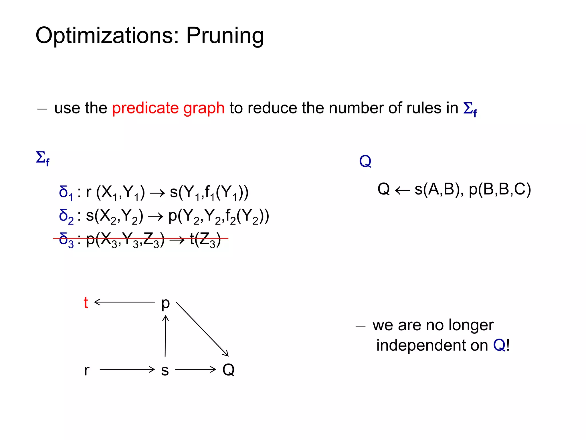
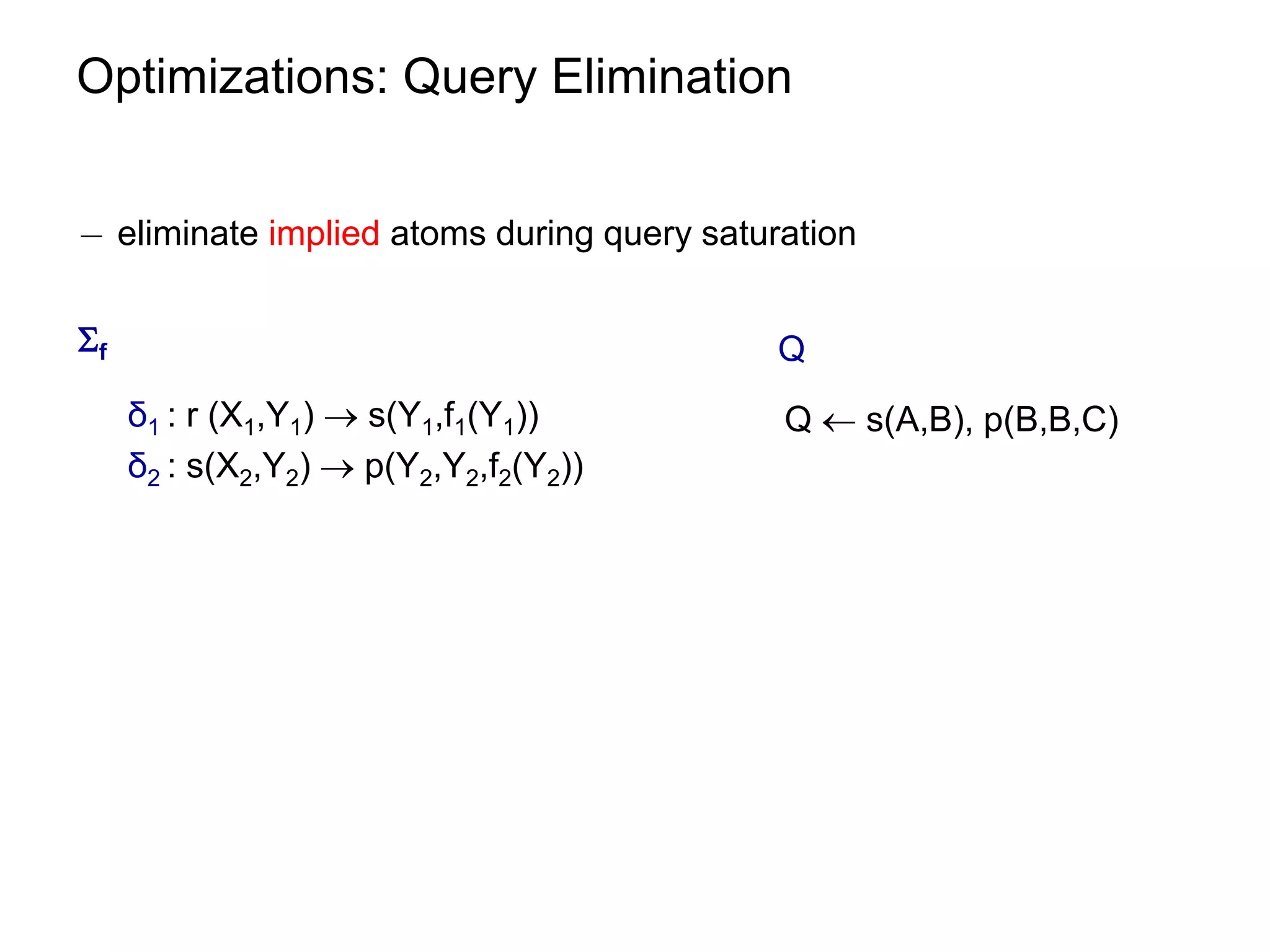
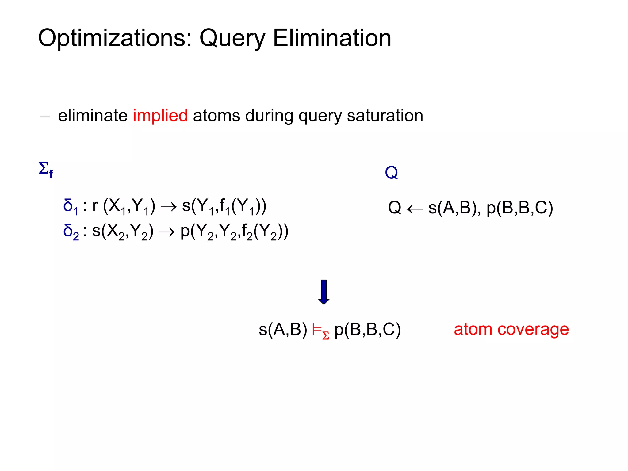
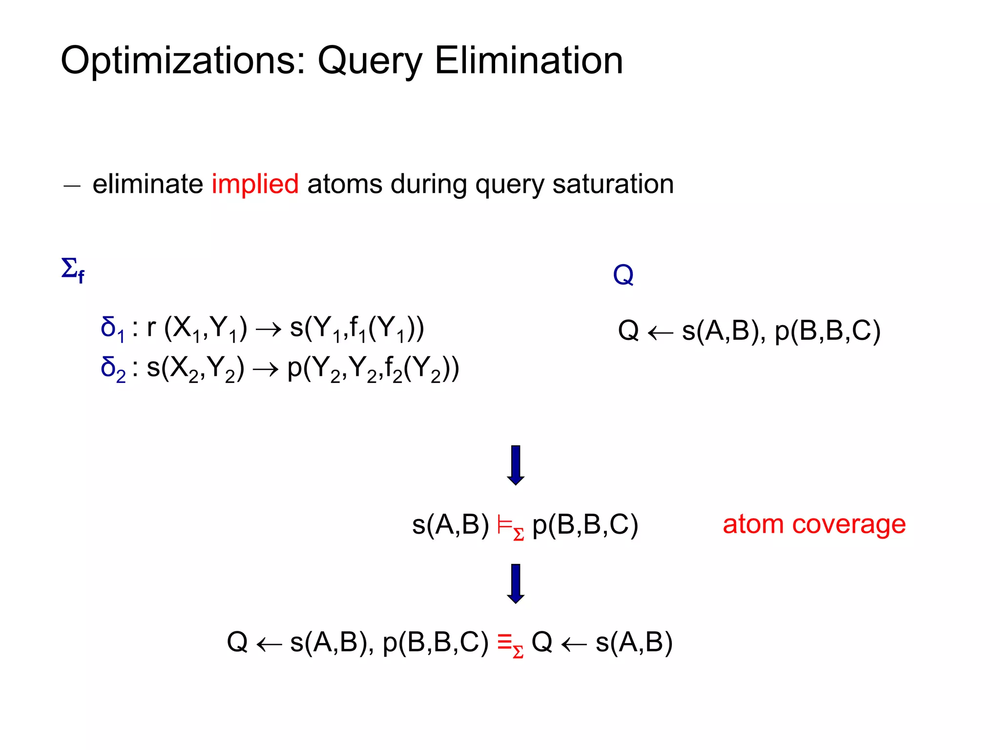
![Optimizations: Query Elimination
¡ atom coverage under linear TGDs can be checked in polynomial time
see paper.
¡ unique elimination strategy (w.r.t. the number of eliminated atoms)
see paper.
¡ given m = |body(ρ)| and n = ||
worst-case size of [f] [ [Q,f] is O((n∙m)m)
worst-case size of Q = <q,π > is O(n+m)m](https://image.slidesharecdn.com/orsivldb11-13154779239988-phpapp01-110908053319-phpapp01/75/Orsi-Vldb11-69-2048.jpg)
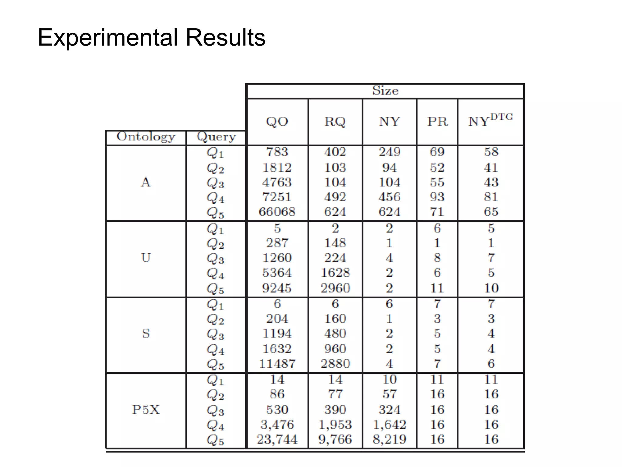
![Discussion
¡ Datalog rewriting is substantially more compact than UCQ rewriting.
¡ Does Datalog improve the end-to-end performance?
¡ Extend the procedure to larger classes of TGDs
guarded TGDs [Cali’ et Al, PODS 09] non FO-rewritable
sticky-join TGDs [Cali’ et Al, VLDB 10]](https://image.slidesharecdn.com/orsivldb11-13154779239988-phpapp01-110908053319-phpapp01/75/Orsi-Vldb11-71-2048.jpg)

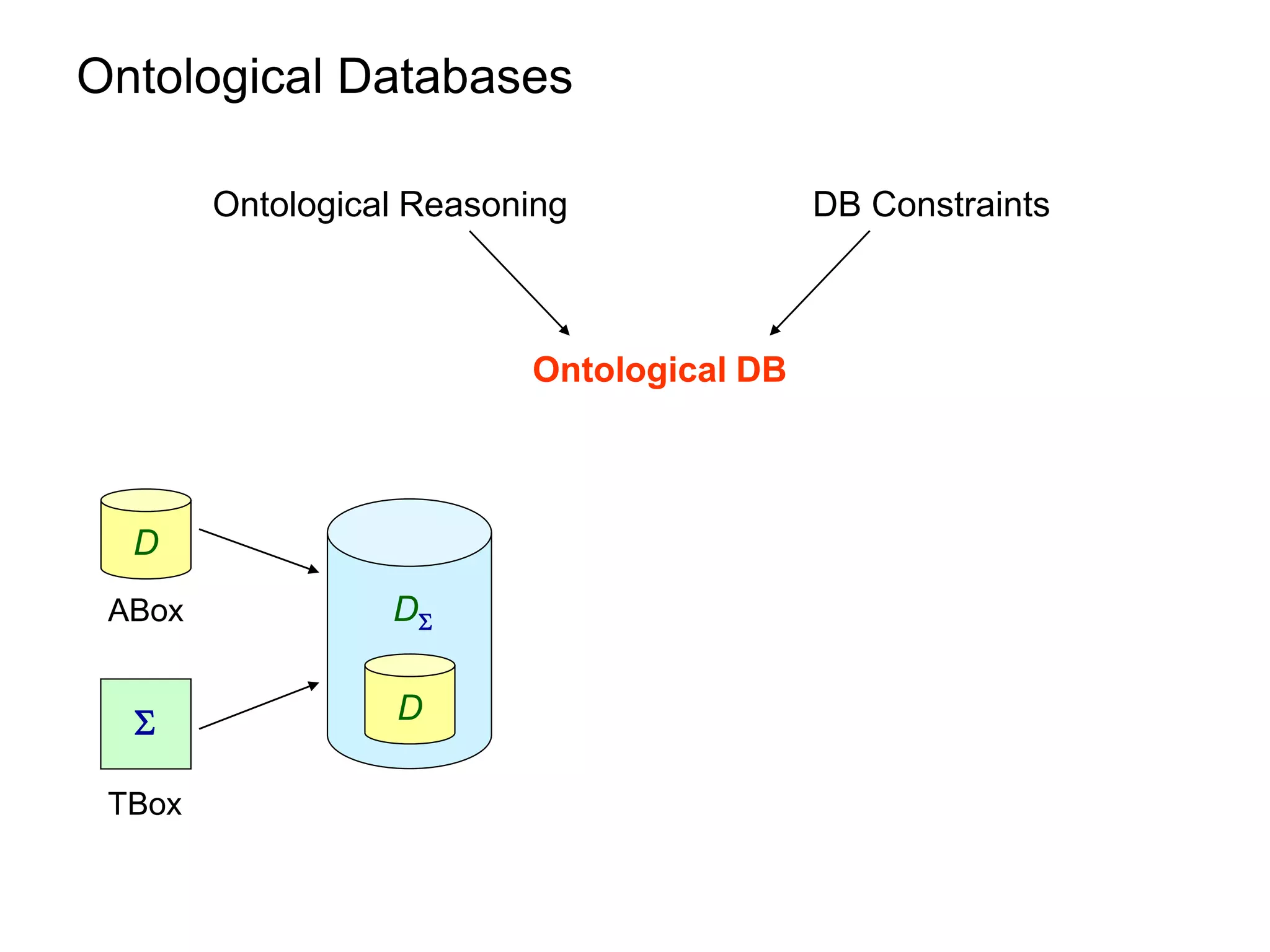
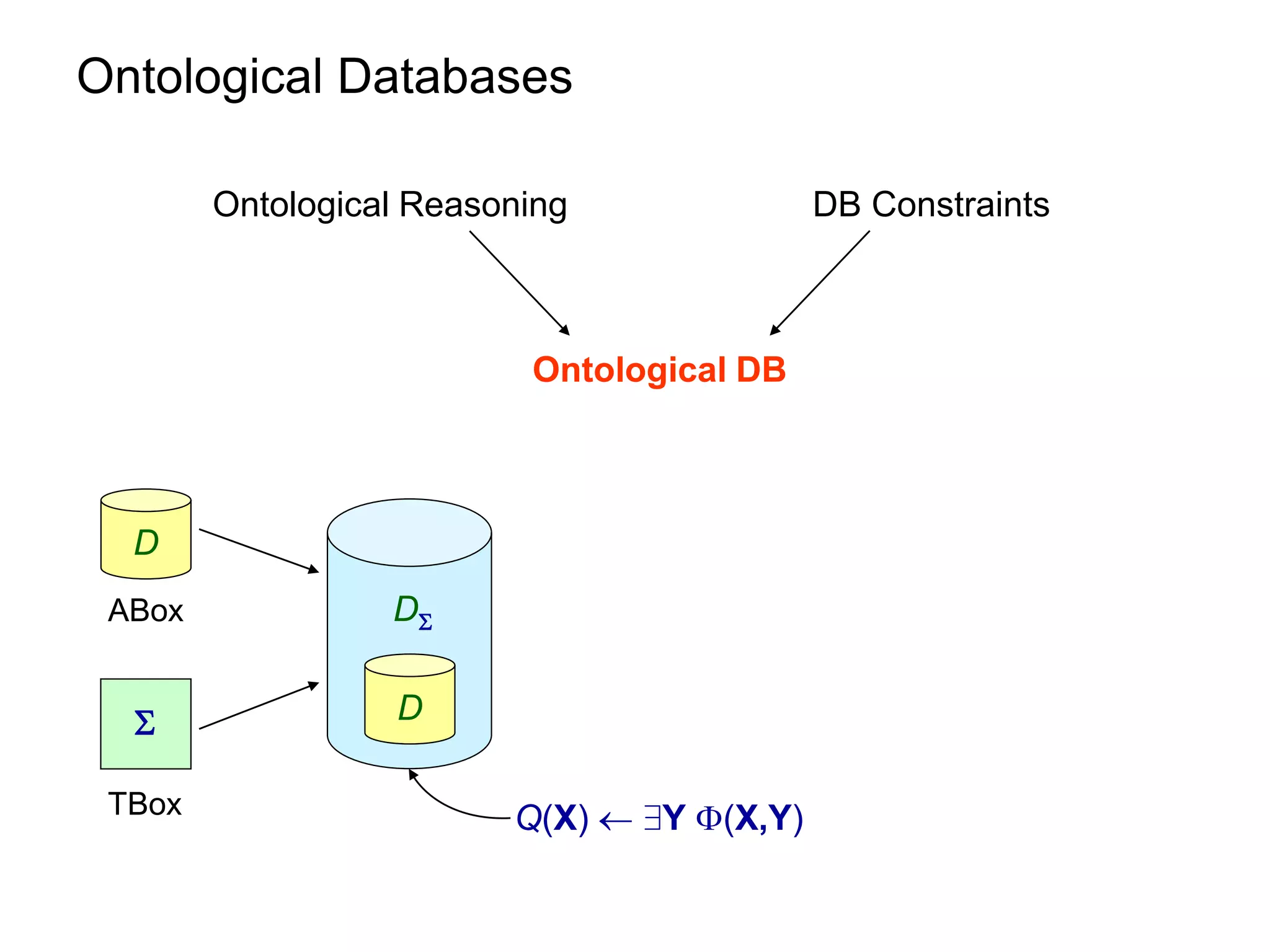
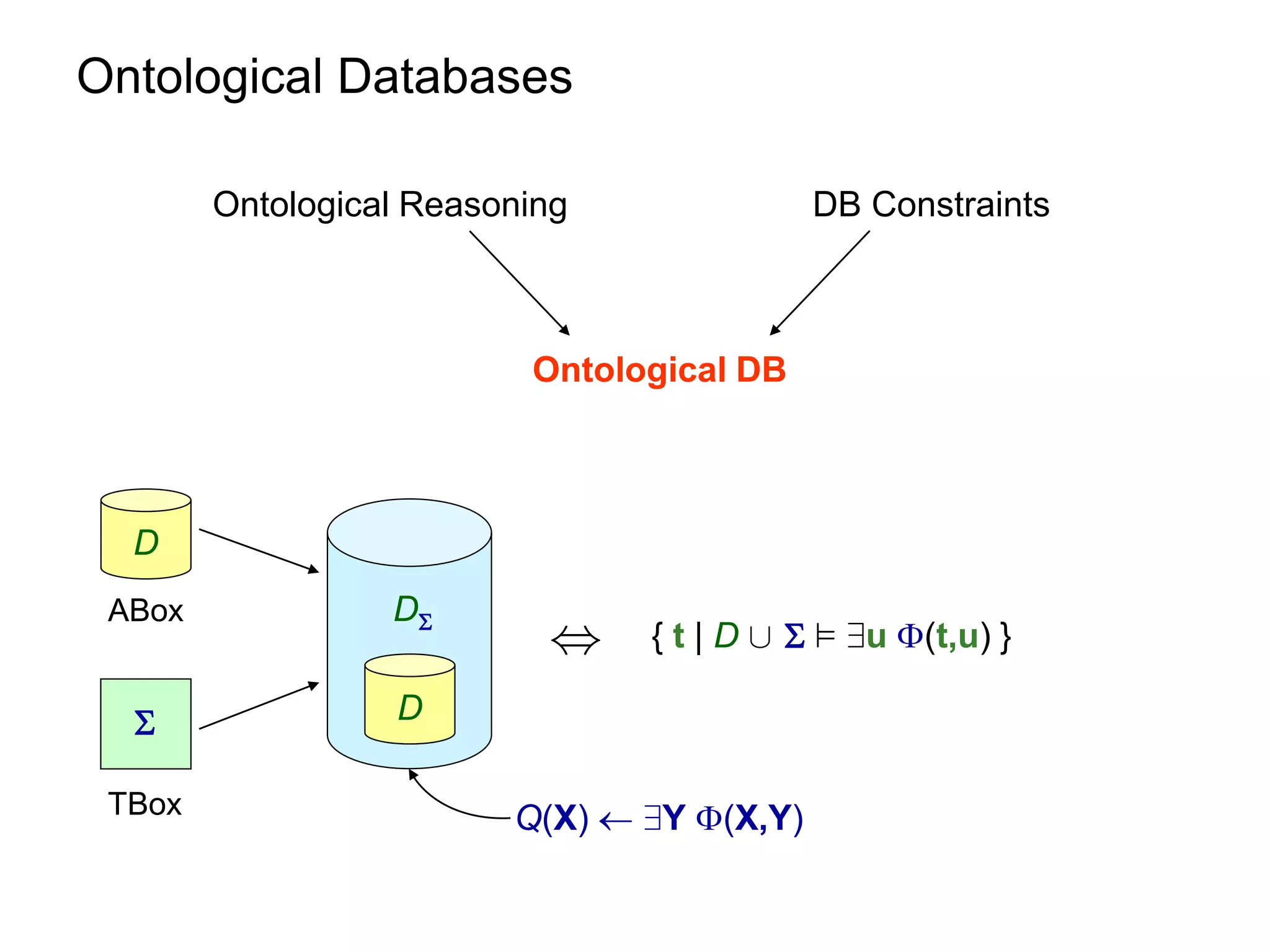
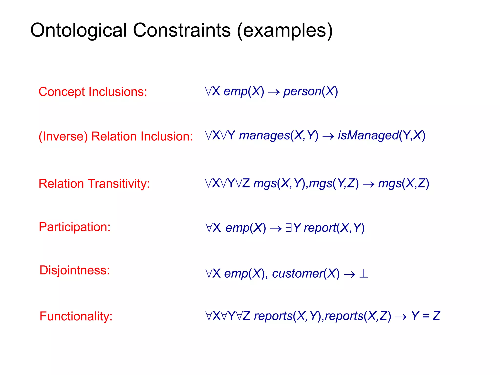
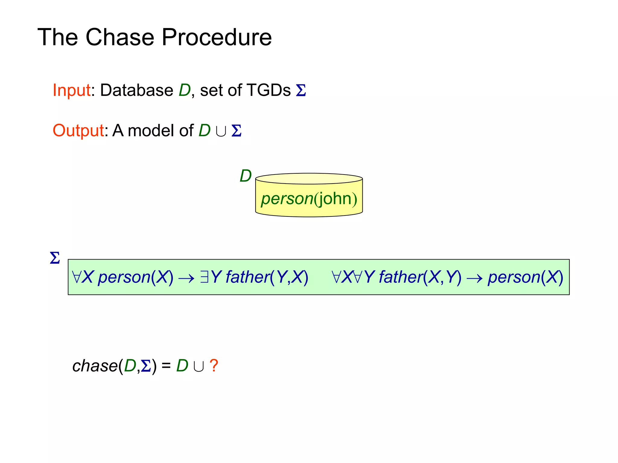
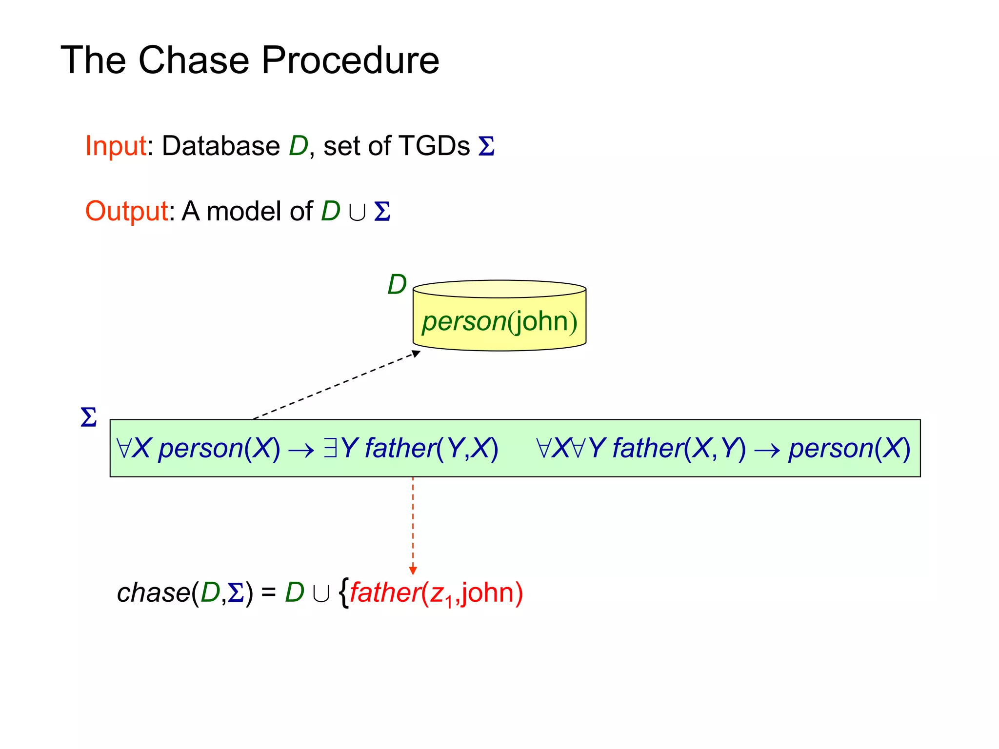
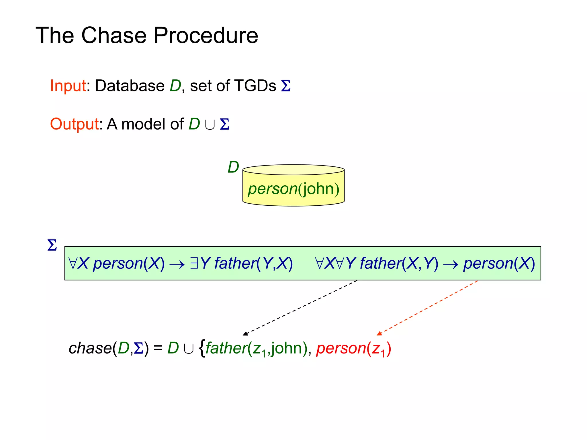
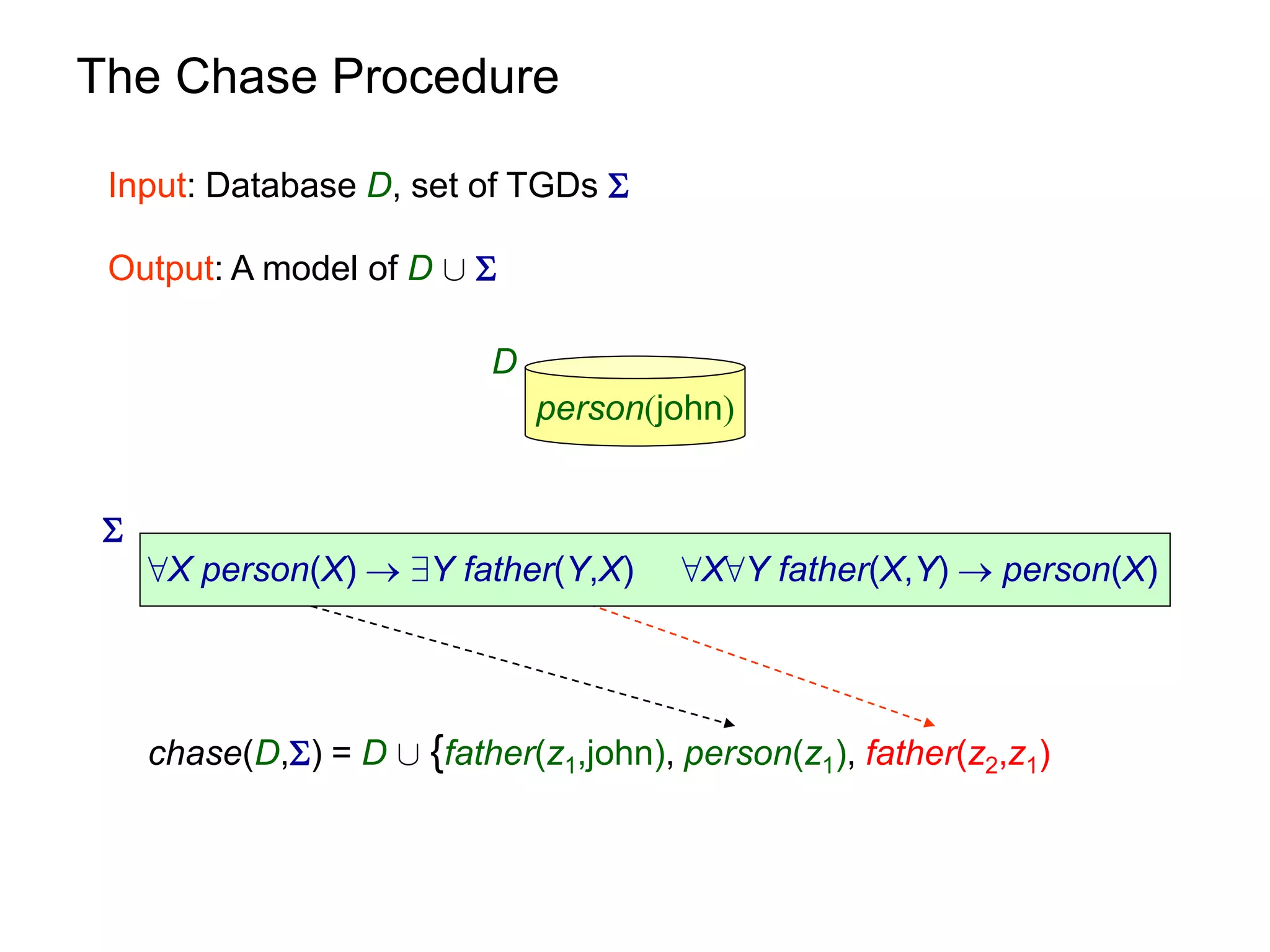
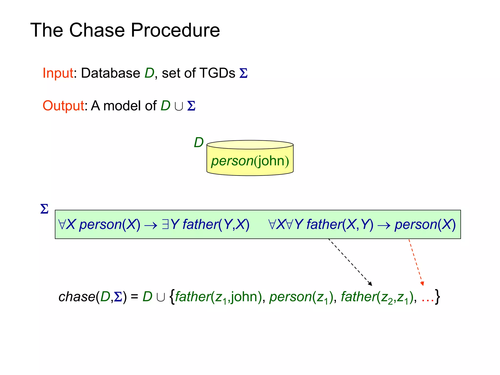
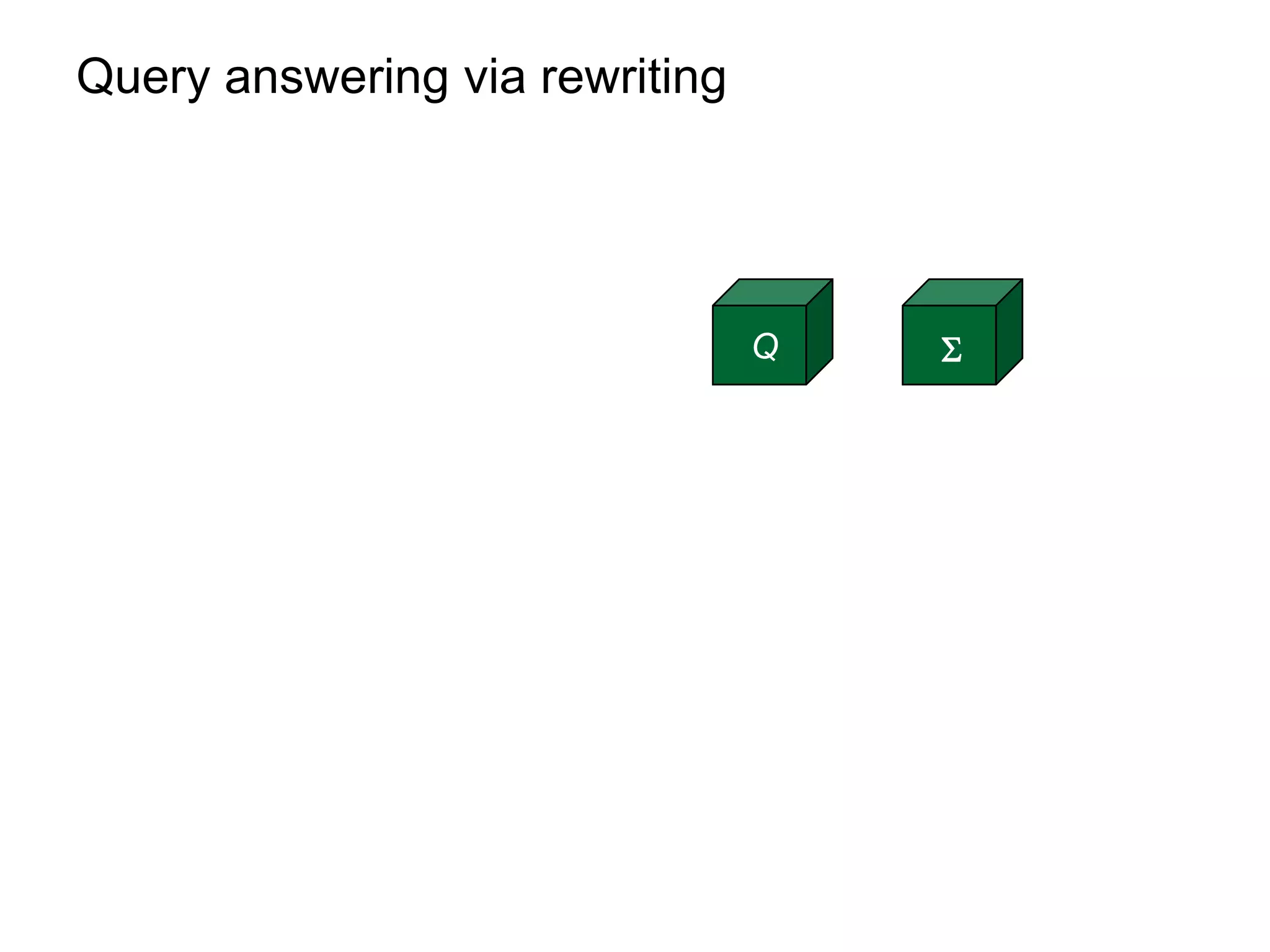
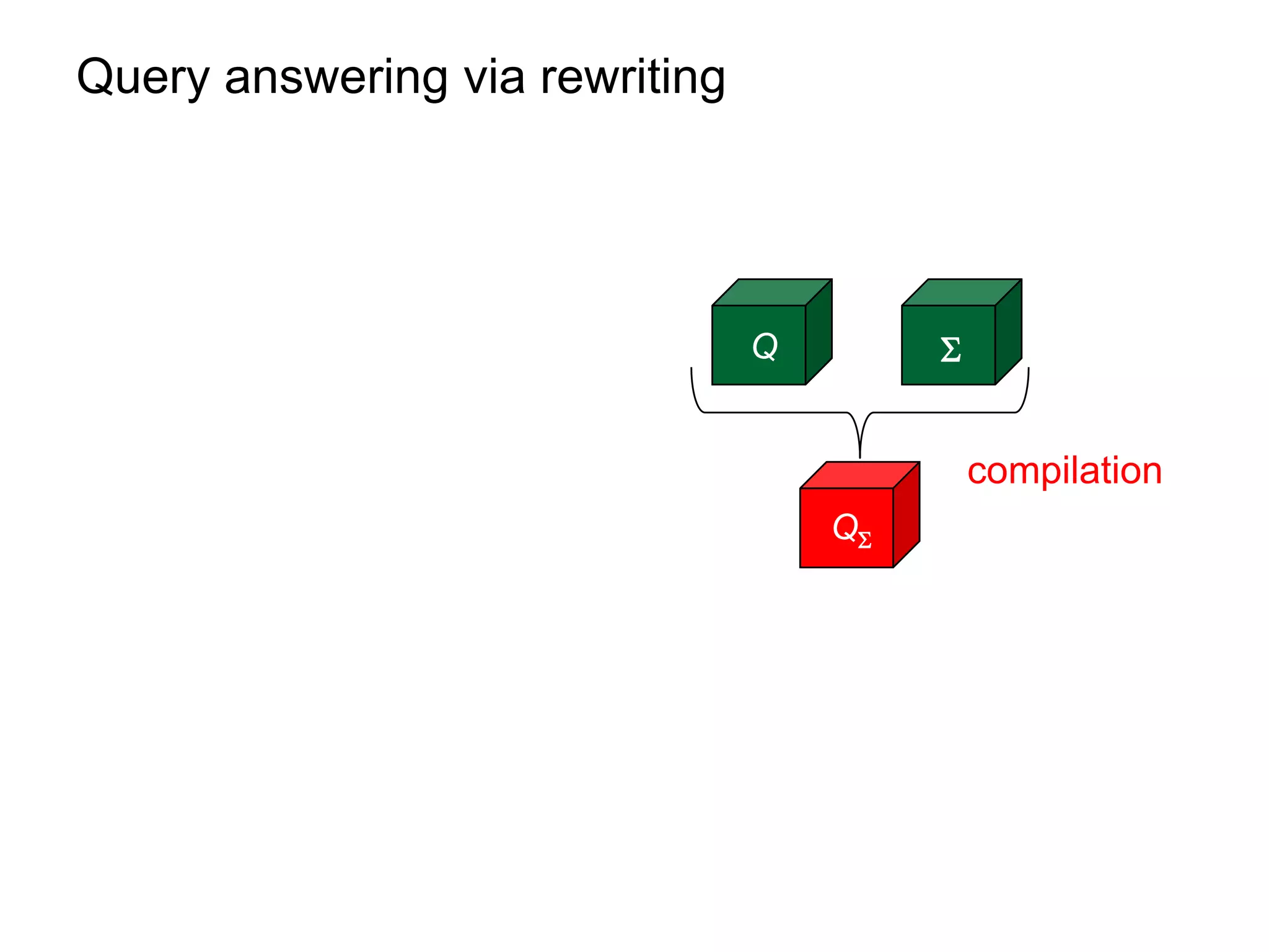
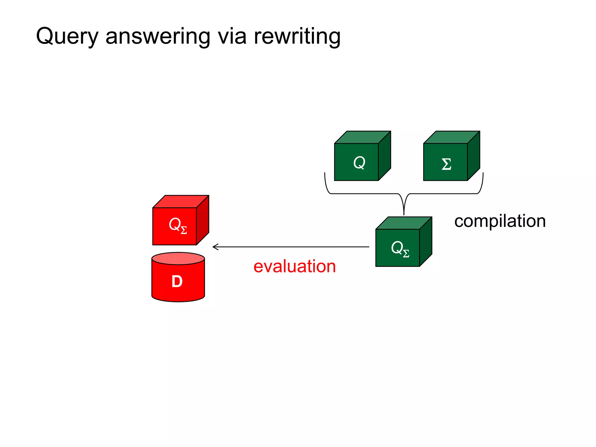
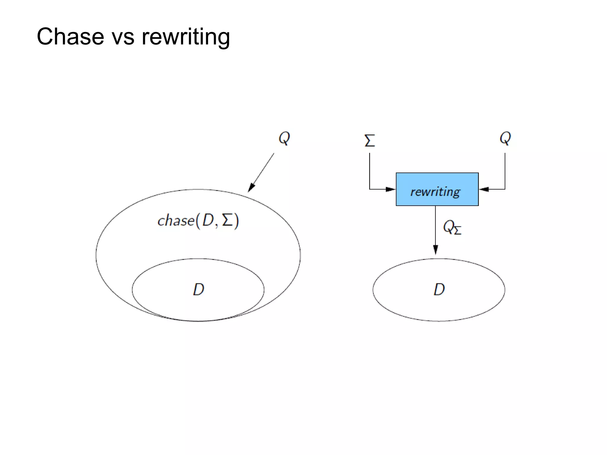
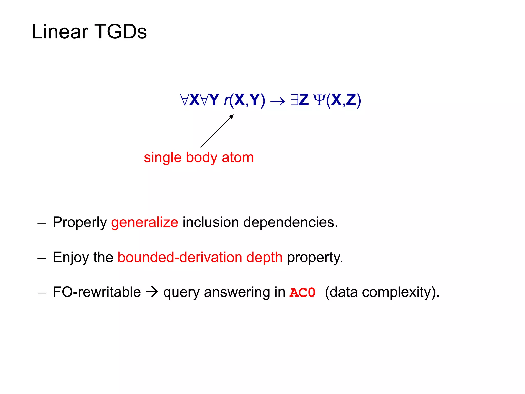
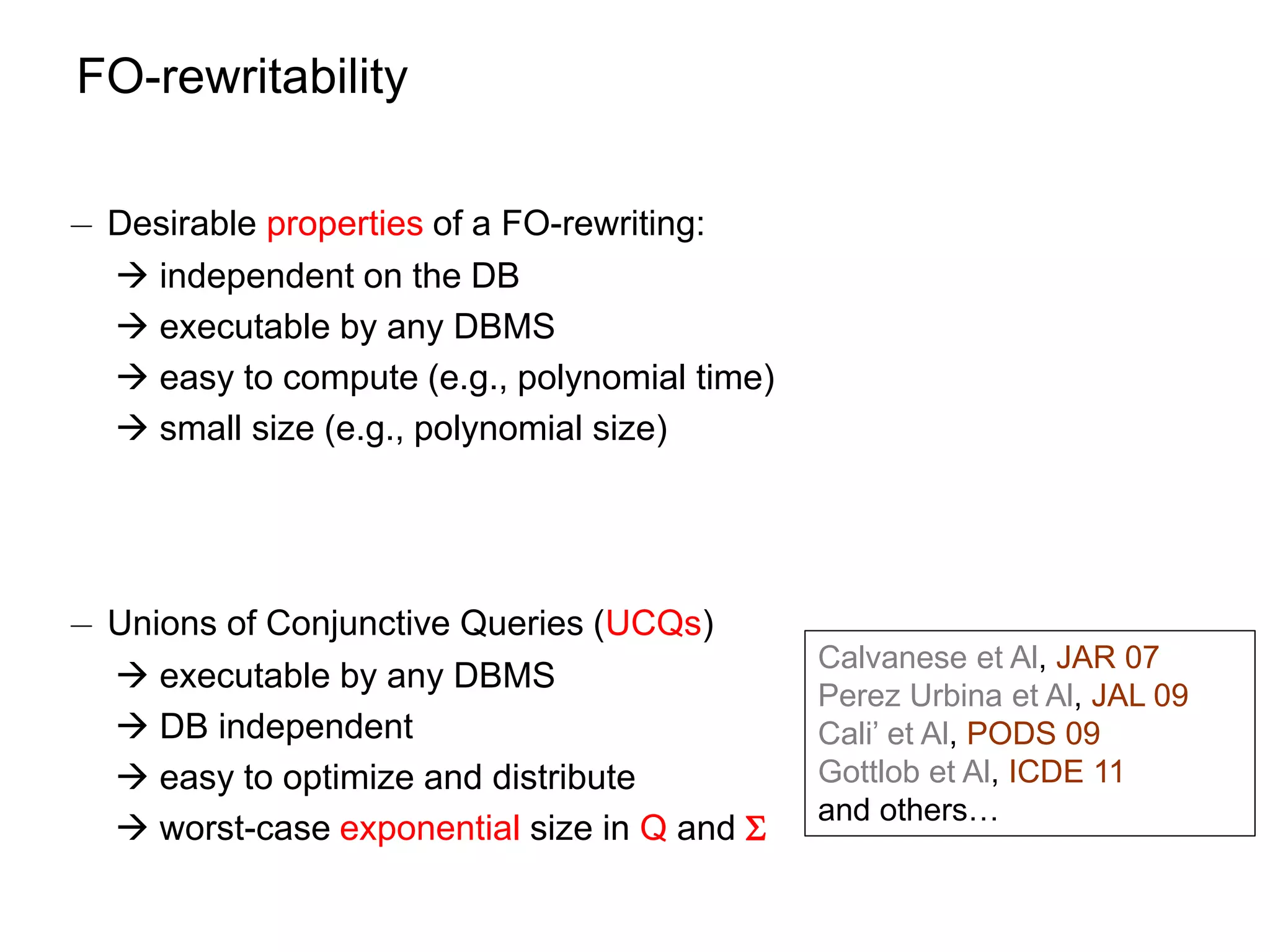
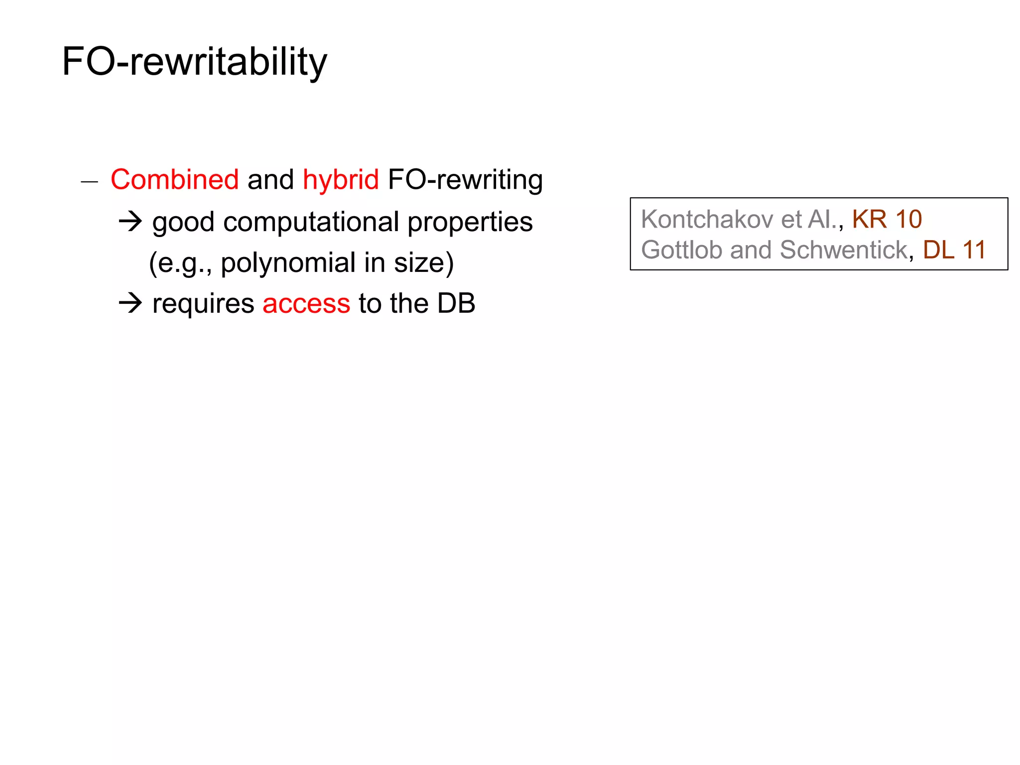
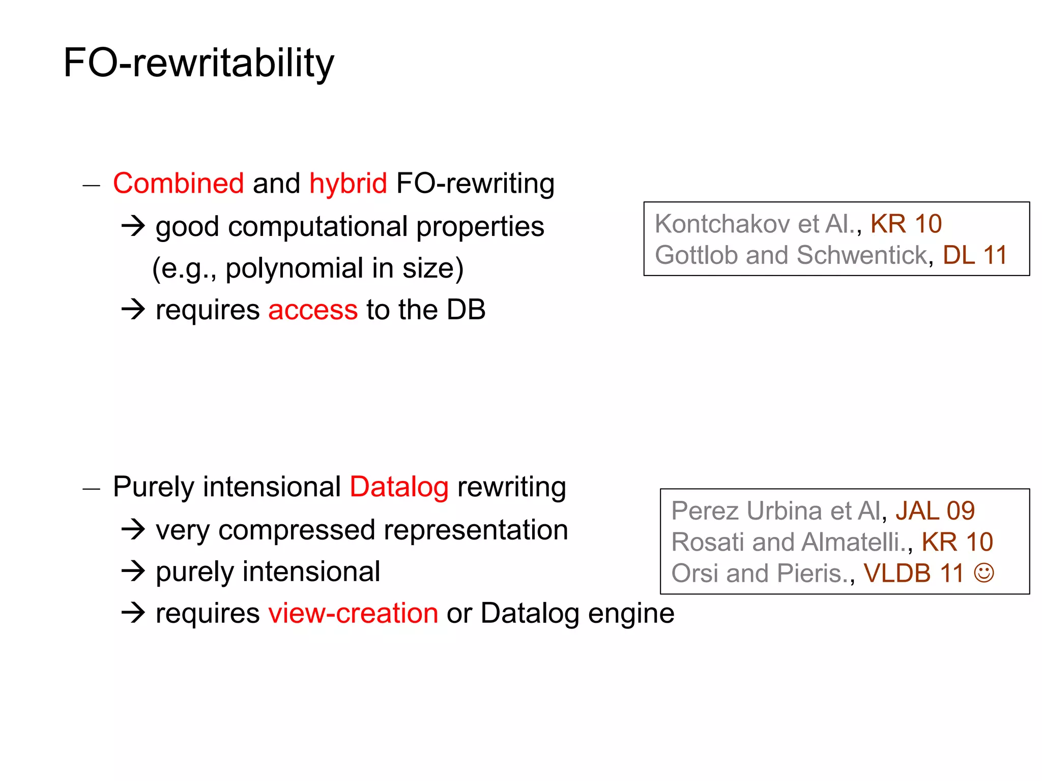
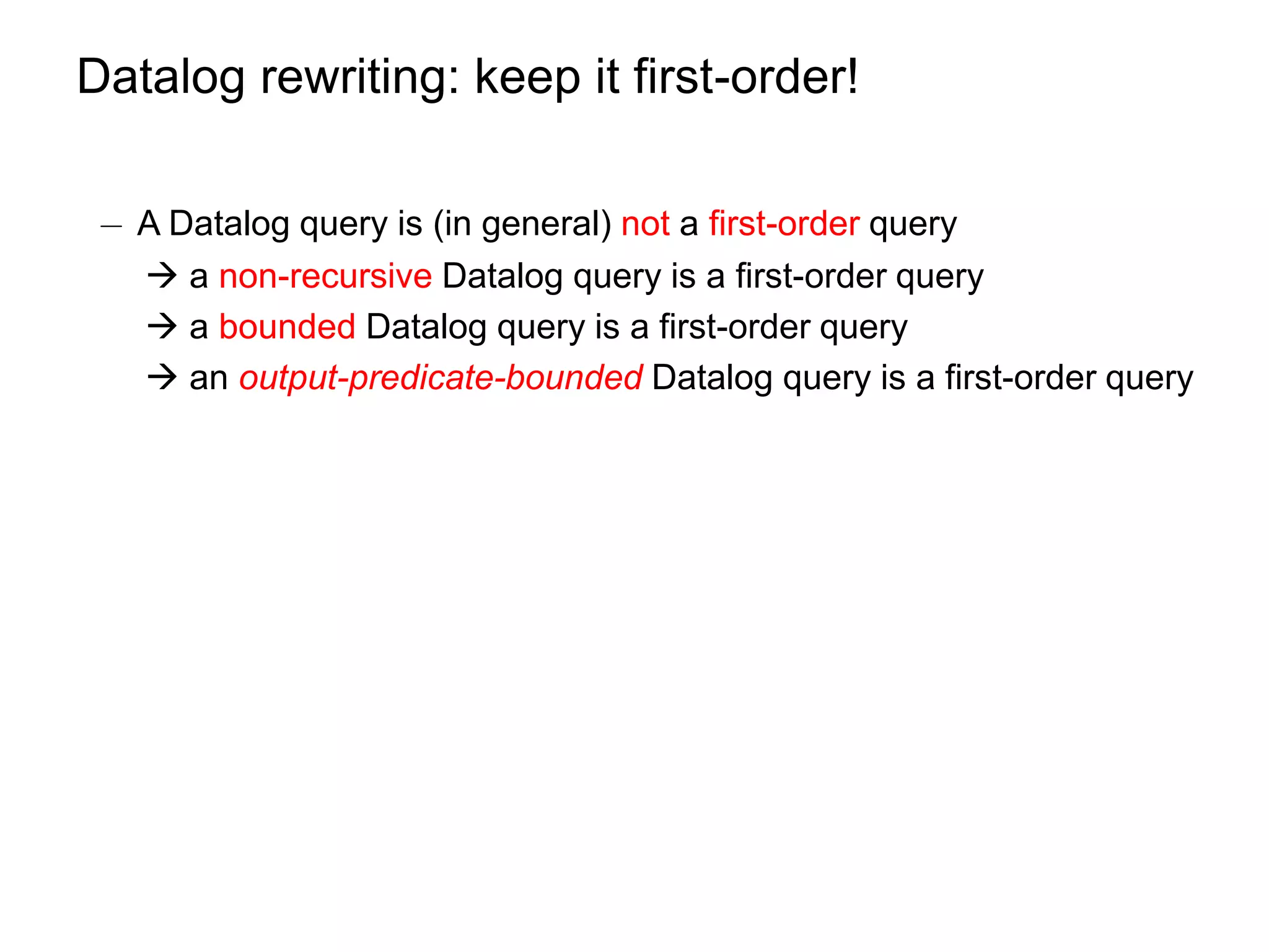
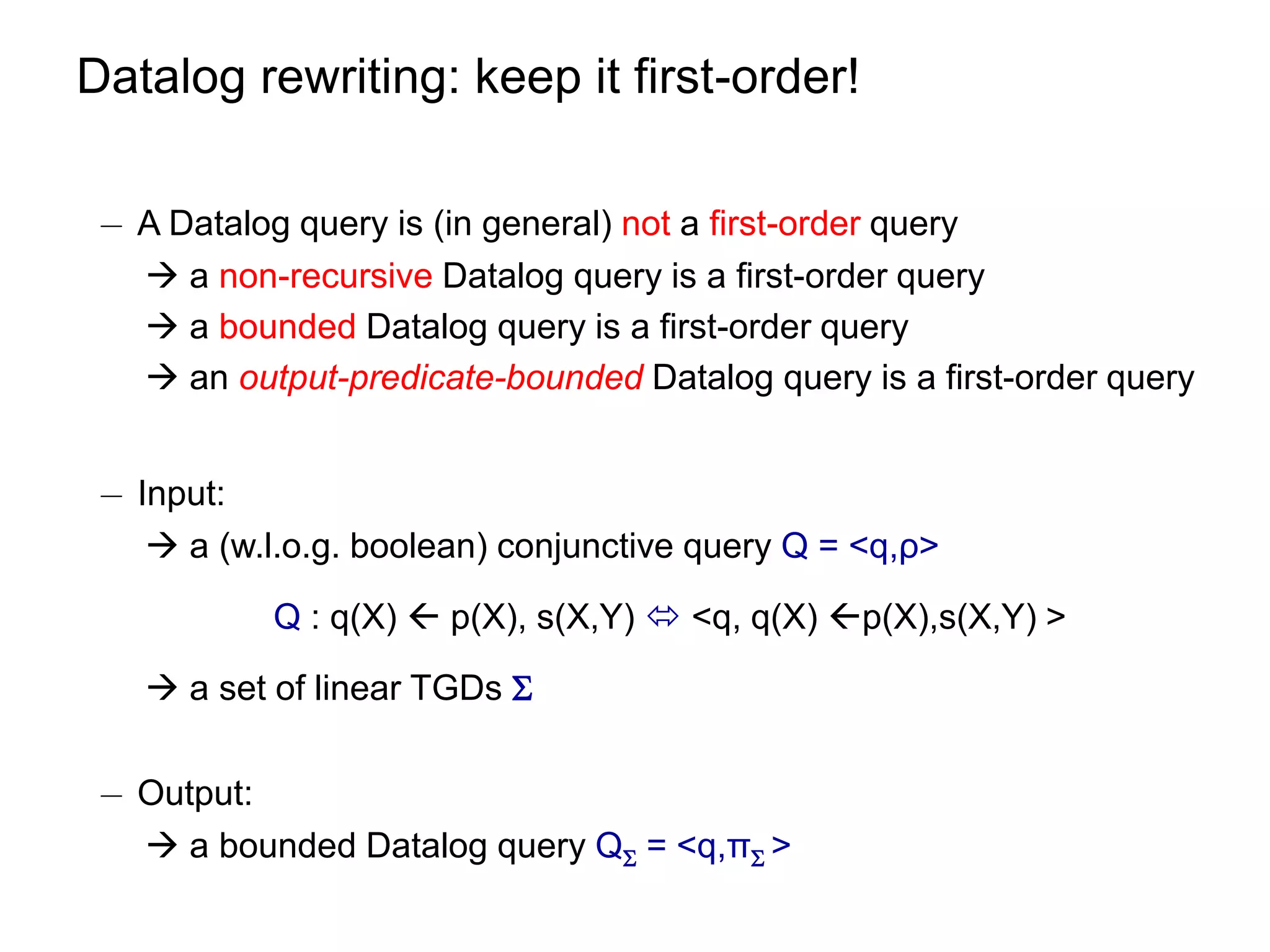
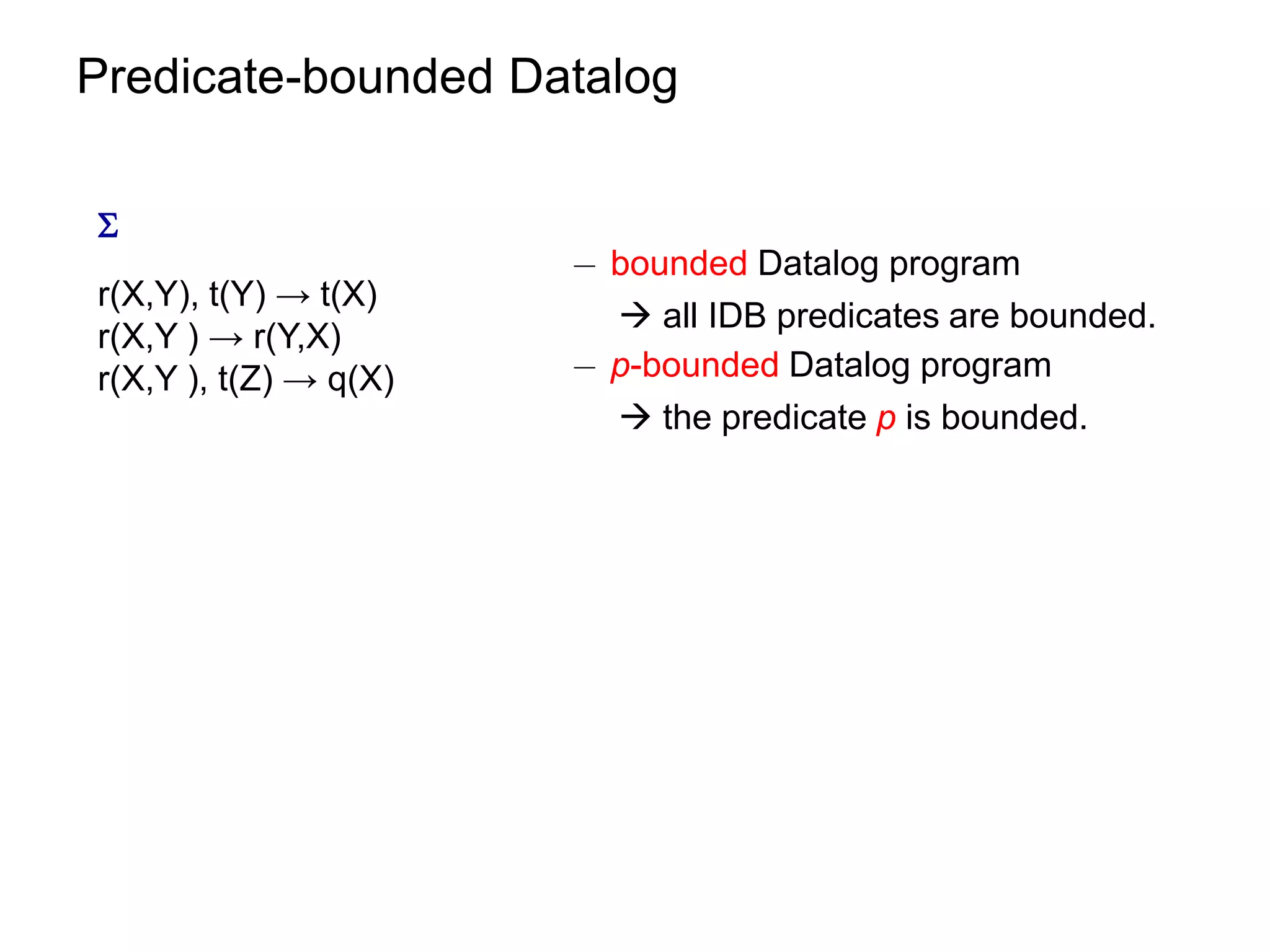
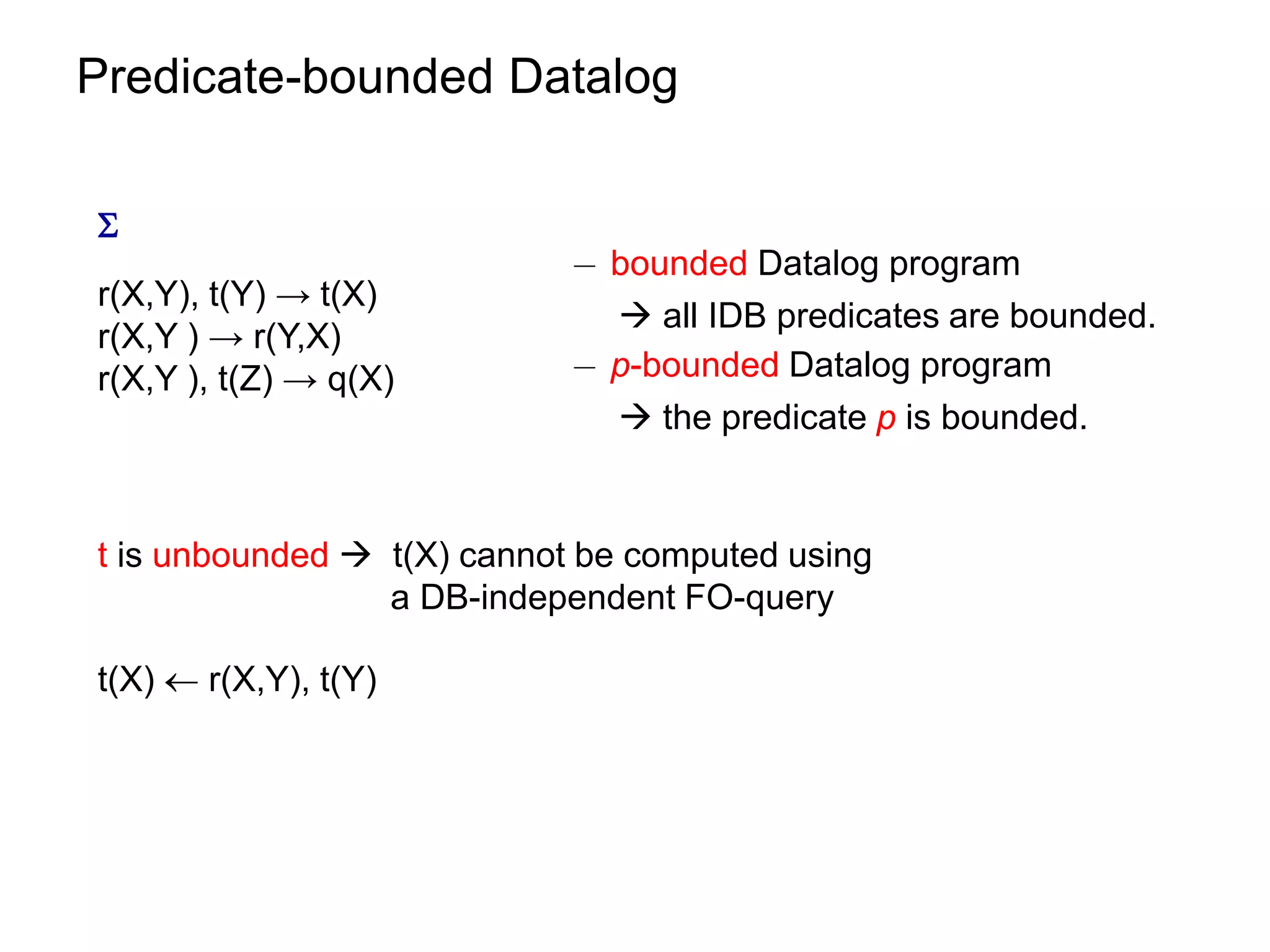
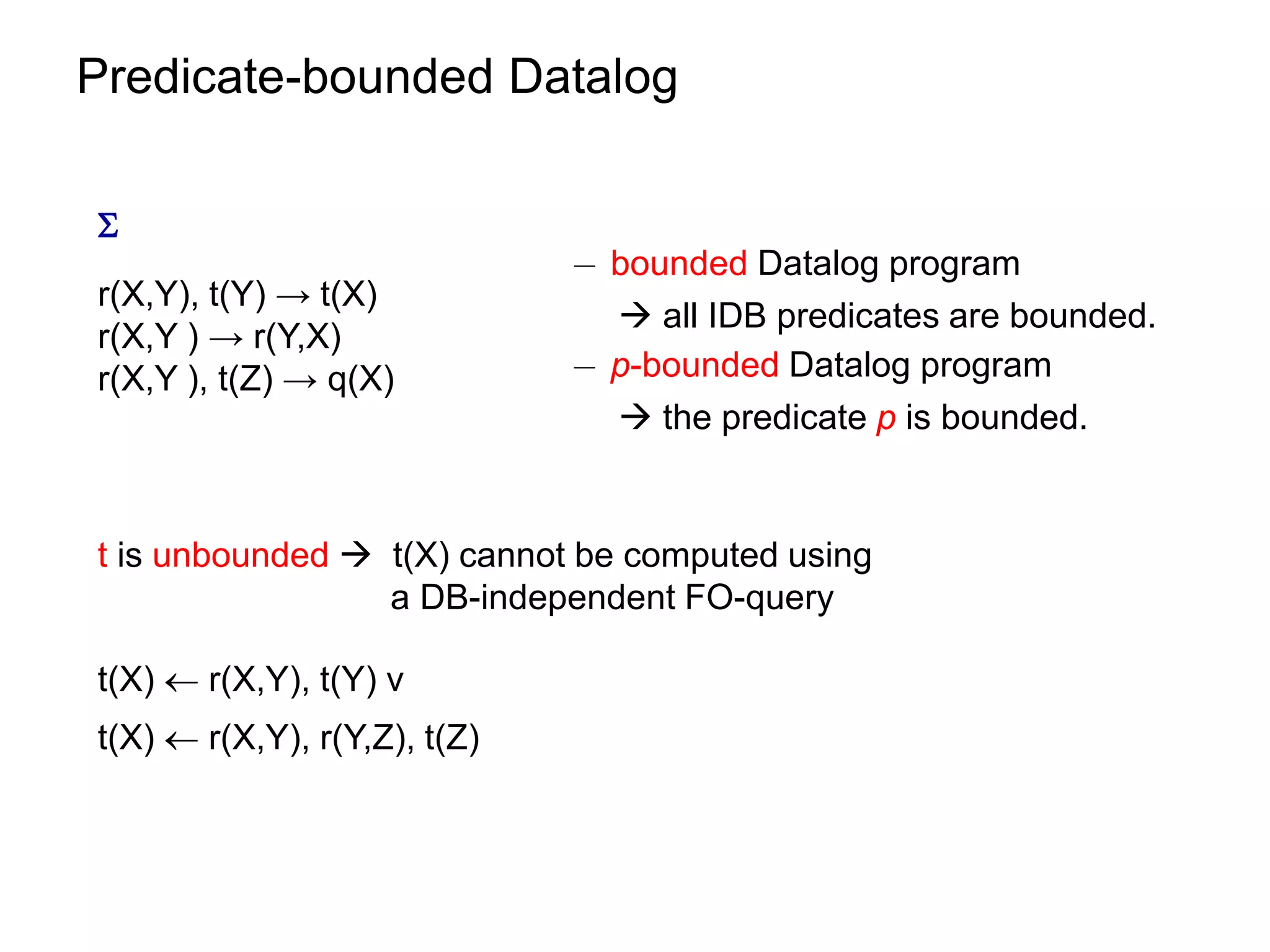
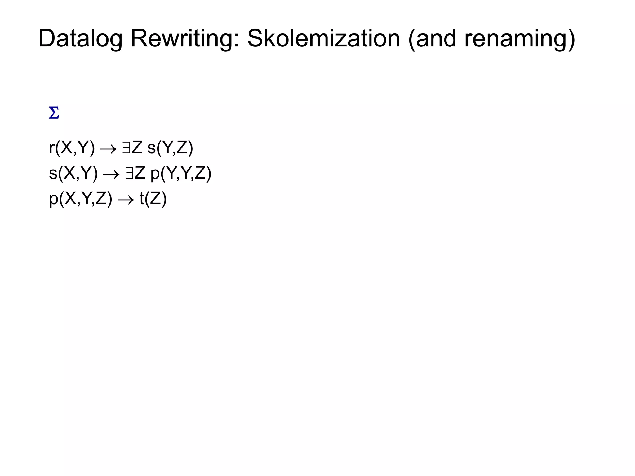
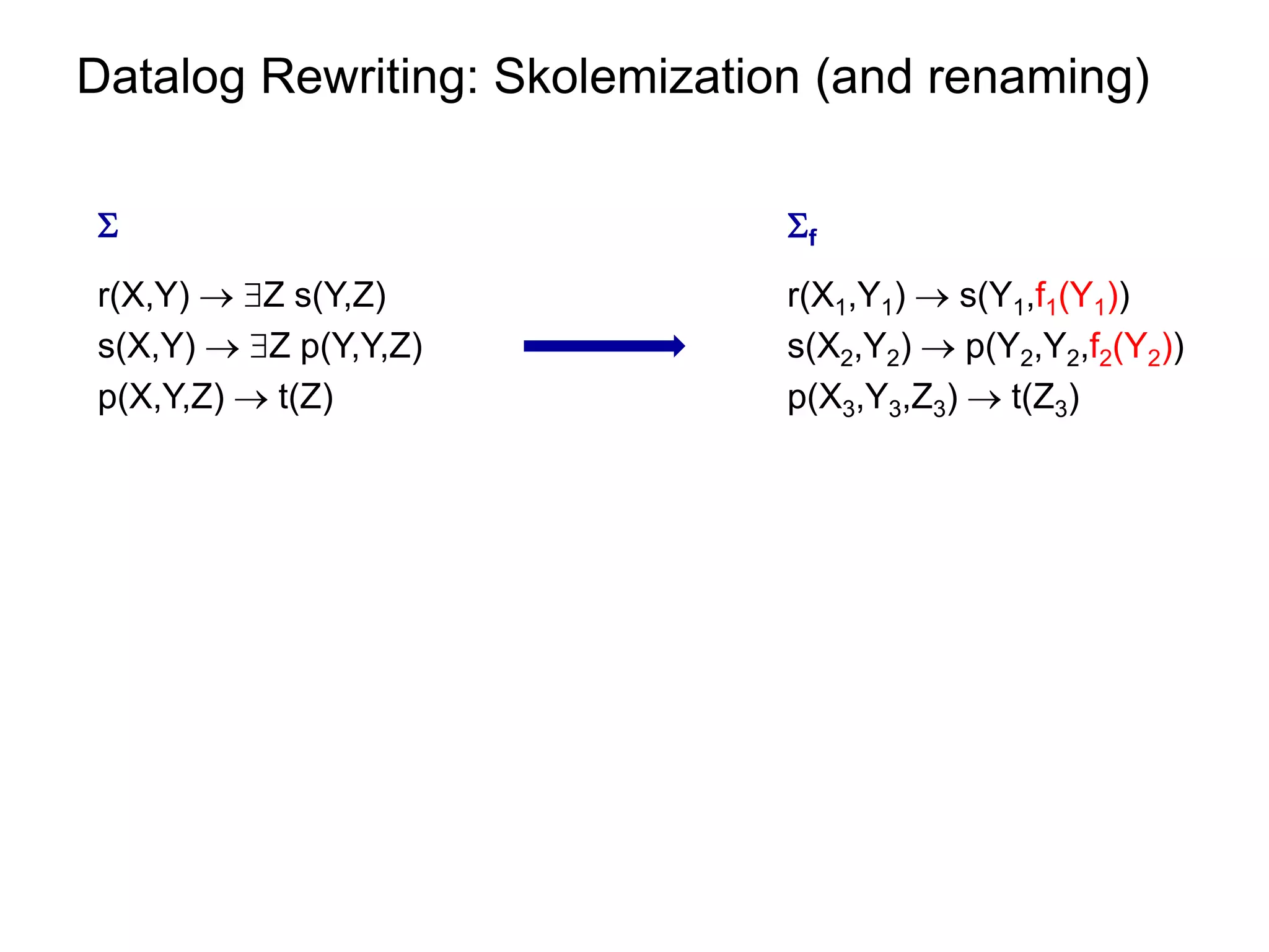
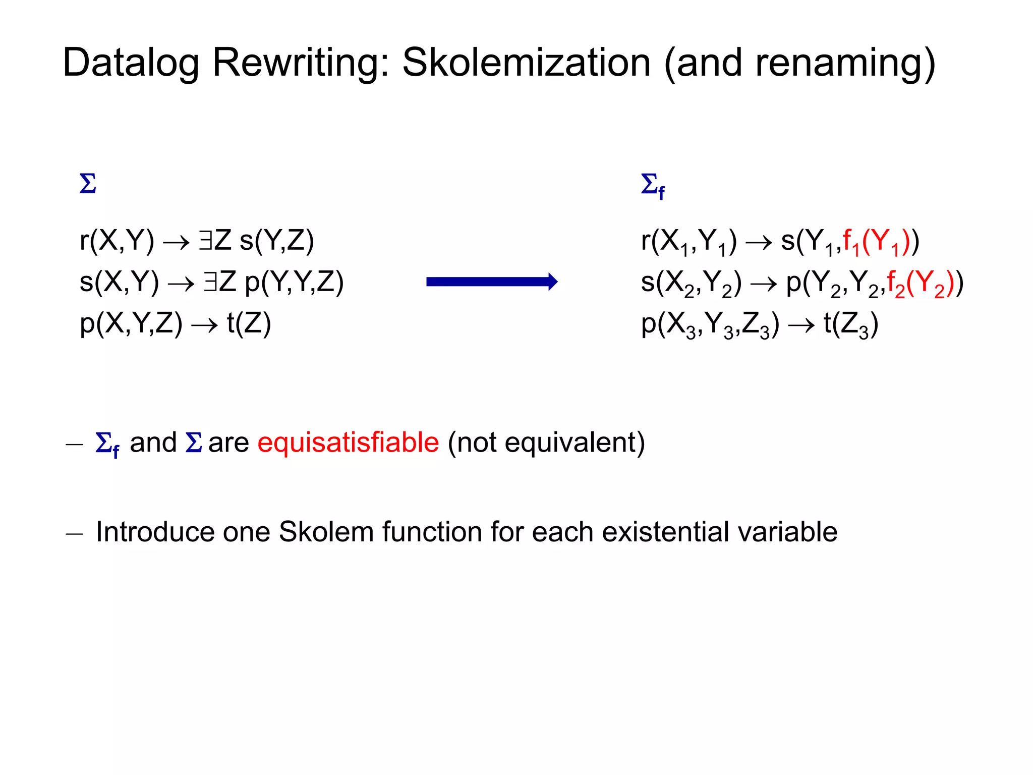
This document summarizes research on optimizing query answering under ontological constraints. Specifically, it discusses: 1) Using the chase procedure to compute a model of the database extended with the ontological constraints, and then evaluating queries over this model. 2) Rewriting queries using the ontological constraints into first-order rewritings that can be evaluated directly over the database. 3) Properties of ontological constraints, like linear tuple-generating dependencies, that ensure the chase terminates and queries can be rewritten as first-order queries, allowing for efficient query evaluation.