OPTIMIZATION TECHNIQUES
IN PHARMACEUTICAL
FORMULATION AND
PROCESSING
Presented by : Areeba
Shafiq
M.phill Pharmaceutics
Scholar (Islamia University
Bahawalpur)
CONTENTS
•Concept of optimization,
• Advantages,
• Optimization parameters,
• Terms (Factor, Effect, Interaction, Confounding, coding),
•Optimization Methodology,
•Experimental Design and its types,
•Computer Software use in Optimization.
CONCEPT OF OPTIMIZATION
•The word optimize simply means to make as perfect, effective, or
functional as possible.
•With respect to drug formulations or pharmaceutical processes,
optimization is a phenomenon of finding the best possible
composition or operating conditions.
• Optimization has been defined as the implementation of systematic
approaches to achieve the best combination of product and/or
process characteristics under a given set of conditions.
ADVANTAGES OF SYSTEMATIC
OPTIMIZATION TECHNIQUES
•Require fewer experiments to achieve an optimum formulation.
•Can trace and rectify a “problem” in a remarkably easier manner.
• Lead to comprehensive understanding of the formulation system.
• Yield the “best solution” in the presence of competing objectives.
•Help in finding the “important” and “unimportant” input variables.
•Tests and improves “robustness” amongst the experimental studies.
•Can change the formulation ingredients or processes independently.
•Aid in determining experimental error and detecting “bad data
points.”
• Can simulate the product or process behavior using model
equation(s).
•Save a significant amount of resources viz. time, effort, materials and
cost.
•Evaluate and improve the statistical significance of the proposed
model(s).
•Can predict the performance of formulations even without preparing
them.
•Detect and estimate the possible interactions and synergies among
variables.
•Facilitate decision–making before next experimentation by response
mapping. Provide reasonable flexibility in experimentation to assess
the product system.
•Can decouple signal from background noise enabling inherent error
estimation.
• Comprehend a process to aid in formulation development and
ensuing scale–up.
•Furnish ample information on formula behavior from one
simultaneous study only.
OPTIMIZATION PARAMETERS
Design and development of any drug formulation or pharmaceutical
process invariably involves several variables.
• Dependant Variables
• Independent Variables
Quantitative Variable Qualitative Variable
Independent Variable
•The input variables, which are directly under the control of the product
development scientist, are known as independent variables
•e.g., drug content, polymer composition, compression force, percentage
of penetration enhancer, hydration volume, agitation speed.
•Such variables can either be quantitative or qualitative.
Quantitative Variable
Quantitative variables are those that can take numeric values (e.g.,
time, temperature, amount of polymer, osmogent, plasticizer,
superdisintegrants) and are continuous.
Qualitative Variable
Qualitative variables ,on the other hand include the type of polymer,
lipid, excipient, or tableting machine. These are also known as
categorical variables. Their influence can be evaluated by assigning
discrete dummy values to them.
Dependent variables
The characteristics of the finished drug product or the in-process
material are known as dependent variables
e.g., drug release profile, percent drug entrapment, pellet size
distribution, moisture uptake.
Popularly termed response variables, these are the measured
properties of the system to estimate the outcome of the experiment.
Usually, these are direct function(s) of any change(s) in the
independent variables.
FACTOR AND EFFECT
Factor
The independent variables, which influence the formulation characteristics
or output of the process, are labeled factors.
The values assigned to the factors are termed levels—e.g., 100 mg and
200 mg are the levels for the factor ,release-rate-controlling polymer in
the compressed matrices.
Effect
The magnitude of the change in response caused by varying the factor
level(s) is termed as an effect. The main effect is the effect of a factor
averaged over all the levels of other factors
INTERACTION
Interaction
An interaction is said to occur when there is “lack of additivity of factor
effects.”
This implies that the effect is not directly proportional to the change in the
factor levels. In other words, the influence of a factor on the response is
nonlinear.
In addition, an interaction may said to take place when the effect of two or
more factors are dependent on each other e.g., the efect of factor A
changes on changing factor B by one unit.
The measured property of the interacting variables depends not only on
their fundamental levels, but also on the degree of interaction between
them. Depending upon whether the change in the response is desired
(positive) or undesired (negative), the phenomenon of interaction may be
CONFOUNDING
• Lack of orthogonality (or independence) is termed confounding or
aliasing.
•When an effect is confounded (or aliased, or mixed up, or equalled),
one cannot assess how much of the observed effect is due to the
factor under consideration.
•Confounding must be assessed qualitatively.
CODING
•The process of transforming a natural variable into a nondimensional
coded variable, Xi , so that the central value of experimental domain is
zero is known as coding (or normalization).
•Generally, the various levels of a factor are designated as –1, 0, and +1,
representing the lowest, intermediate (central), and highest factor levels
investigated, respectively.
•For instance, if sodium carboxymethyl cellulose, a hydrophilic polymer, is
studied as a factor in the range of 120–240 mg, then codes –1 and +1
signify 120 mg and 240 mg amounts, respectively. The code 0 would
represent the central point at the arithmetic mean of the two extremes—
i.e., 180 mg.
DRUG DELIVERY OPTIMIZATION : DOE
METHODOLOGY
An experimental approach to DoE optimization of DDS comprises several
phases. Broadly, these phases can be sequentially summed up in seven
salient steps.
Seven-Step ladder for optimizing drug delivery system
STEP I :Objective
The optimization study begins with Step I, where an endeavor is made
to ascertain the initial drug delivery objective(s) in an explicit manner.
Various main response parameters, which closely and pragmatically
epitomize the objective(s), are chosen for the purpose.
STEP 2 :Factor Studies
The experimenter has several potential independent product and/or
process variables to choose from. By executing a set of suitable
screening techniques and designs, the formulator selects the “vital
few” influential factors among the possible “so many” input variables.
Following selection of these factors, a factor influence study is carried
out to quantitatively estimate the main effects and interactions.
Before going to the more detailed study, experimental studies are
undertaken to defi ne the broad range of factor levels as well.
STEP 3:Response Surface Modeling and Experimental Designs
During Step III, an apposite experimental design is worked out on the
basis of the study objective(s), and the number and the type of
factors, factor levels, and responses being explored. Working details
on variegated vistas of the experimental designs, customarily
required to implement DoE optimization of drug delivery, have been
elucidated in the subsequent section.
Afterwards, response surface modeling (RSM) is characteristically
employed to relate a response variable to the levels of input variables,
and a design matrix is generated to guide the drug delivery scientist
to choose optimal formulations.
Step IV: Formulation of DDS and Their Evaluation
In Step IV, the drug delivery formulations are experimentally prepared
according to the approved experimental design, and the chosen
responses are evaluated.
Step V: Computer-Aided Modeling and Optimization
In Step V, a suitable mathematical model for the objective(s) under
exploration is proposed, the experimental data thus obtained are
analyzed accordingly, and the statistical signifi cance of the proposed
model discerned. Optimal formulation compositions are searched
within the experimental domain, employing graphical or numerical
techniques. h is entire exercise is invariably executed with the help of
pertinent computer software.
Step VI: Validation of Optimization Methodology
Step VI is the penultimate phase of the optimization exercise,
involving validation of response prognostic ability of the model put
forward. Drug delivery performance of some studies, taken as the
checkpoints, is assessed vis-à-vis that predicted using RSM, and the
results are critically compared.
Step VII: Scale-Up and Implementation in Production Cycle
Fınally, during Step VII, which is carried out in the industrial milieu,
the process is scaled up and set forth ultimately for the production
cycle.
EXPERIMENTAL DESIGN AND ITS
TYPES
An experimental design is the statistical strategy for organizing the
experiments in such a manner that the required information is obtained as
efficiently and precisely as possible.
Runs or trials are the experiments conducted according to the selected
experimental design.Such DoE trials are arranged in the design space so that
the reliable and consistent information is attainable with minimum
experimentation. The layout of the experimental runs in a matrix form,
according to the experimental design, is known as the design matrix.
The choice of design depends upon the
oproposed model,
othe shape of the domain,
oand the objective of the study.
Primarily, the experimental (or statistical) designs are based on the
principles of :
o Randomization (i.e., the manner of allocations of treatments to the
experimental units),
o Replication (i.e., the number of units employed for each treatment),
oAnd error control or local control (i.e., the grouping of specific types
of experiments to increase the precision).
TYPES OF EXPERIMENTAL DESIGN
There are numerous types of experimental designs. Various
commonly employed experimental designs for RSM, screening, and
factor-infl uence studies in pharmaceutical product development
are
a. factorial designs b. fractional factorial designs
c. Plackett–Burman designs d. star designs
e. central composite designs f. Box–Behnken designs
g. center of gravity designs h. equiradial designs
i. mixture designs j. Taguchi designs
k. optimal designs l. Rechtschaffner designs
m. Cotter designs
1.FACTORIAL DESIGN
Factorial designs (FDs) are very frequently used response surface
designs
A factorial experiment is one in which all levels of a given factor are
combined with all levels of every other factor in the experiment.
These are generally based upon first-degree mathematical models.
Full FDs involve studying the effect of all the factors (k) at various
levels (x), including the interactions among them, with the total
number of experiments being Xk
FDs can be investigated at either two levels (2k FD) or more
than two levels. If the number of levels is the same for each
factor in the optimization study, the FDs are said to be
symmetric, whereas in cases of a different number of levels for
2K factorial designs.
The two-level FDs are the simplest form of orthogonal design,
commonly employed for screening and factor influence studies.
They involve the study of k factors at two levels only—i.e., at high (+)
and low (–) levels. The simplest FD involves investigation of two
factors at two levels only.
Characteristically, these represent first-order models with linear
response.
Higher level factorial designs.
•FDs at three or more number of levels are employed mainly for
response surface optimization. Simple to generate, these designs can
detect and estimate nonlinear or quadratic effects.
• The main strength of the design is orthogonality, because it allows
independent estimation of the main effects and interactions.
• On the other hand, the major limitation associated with high-level
FDs is the increased number of experiments required with the
increase in the number of factors (k).
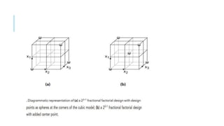
2.FRACTIONAL FACTORIAL DESIGN
In a full FD, as the number of factors or factor levels increases, the
number of required experiments exceeds manageable levels.
Also, with a large number of factors, it is possible that the highest
order interactions have no significant effect.
In such cases, the number of experiments can be reduced in a
systematic way, with the resulting design called fractional factorial
designs (FFD) or sometimes partial factorial designs.
An FFD is a finite fraction (1/xr )of a complete or “full” FD, where r is
the degree of fractionation and xk-r is the total number of
experiments required.
For a two-level, three-factor design, a full FD will require 2³—i.e.,
eight experiments and seven effects are determined. Out of these
seven effects, there are three main effects, and the other four effects
are due to the interactions among the three factors.
An FFD with r = 1, on the other hand, will require only 2³– ¹, i.e., four
experiments and a total of three effects are estimated. However,
these three effects are the combined effects of factors and
interactions.
3.PLACKETT–BURMAN DESIGNS
Plackett–Burman designs (PBD) are special two-level FFDs used
generally for screening of K—i.e., N–1 factors, where N is a multiple
of 4.
Also known as Hadamard designs or symmetrically reduced 2k-r FDs,
the designs can easily be constructed employing a minimum number
of trials.
For instance, a 30-factor study can be accomplished using only 32
experimental runs.
4.STAR DESIGN
Because FDs do not allow detection of curvature unless more than
two levels of a factor are chosen, a star design can be used to
alleviate the problem and provide a simple way to fit a quadratic
model.
The number of required experiments in a star design is given by 2k +
1.
A central experimental point is located from which other factor
combinations are generated by moving the same positive and negative
distance (= step size, α).
For two factors, the star design is simply a 2² FD rotated over 45° with
an additional center point . The design is invariably orthogonal and
The diagrammatic representation of a star design with an additional
center point derived from the factorial by rotation over 45ͦ
5.CENTRAL COMPOSITE DESIGN
• For nonlinear responses requiring second-order models, central
composite designs (CCDs) are the most frequently employed.
•Also known as the Box–Wilson design
•The “composite design” contains an imbedded (2K ) FD or (2k-r) FFD,
augmented with a group of star points (2k) and a “central” point.
• The star points allow estimation of curvature and establish new extremes
for the low and high settings for all the factors.
•Hence, CCDs are second-order designs that effectively combine the
advantageous features of both FDs (or FFDs) and the star design.
• The total number of factor combinations in a CCD is given by 2K + 2k +
1.
6.BOX BEHNKEN DESIGN
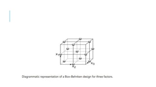
•A specially made design, the Box–Behnken design (BBD), requires only
three levels for each factor—i.e., –1, 0, and +1.
• A BBD is an economical alternative to CCD.
•It overcomes the inherent pitfalls of the CCDs
• This is an independent quadratic design, in that it does not contain an
embedded FD or FFD. Although BBD is also called orthogonal balanced
incomplete block design, it has limited capability for orthogonal
blocking in comparison to the CCDs.
• The design is rotatable (or nearly rotatable).
• The BBDs are also popularly used for response surface optimization of
drug delivery systems.
7.CENTER OF GRAVITY DESIGNS
•These designs are modifications of CCD.
•Retaining the advantages of CCD, these designs further reduce the total
number of experiments to 4k + 1.
• The experiments start with a midpoint, which usually lies in the
factorial region.
•From this midpoint (i.e., center of gravity), at least four points are
decided on each coordinate axis in such a way that the resulting
geometric space becomes as large as possible.
•Despite the broader geometric space, the designs include only
meaningful experiments.
•Such designs have been employed to optimize various DDS quite
frequently.
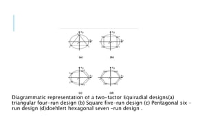
8.EQUIRADIAL DESIGNS
•Equiradial designs are first-degree response surface designs, consisting
of N points on a circle around the center of interest in the form of a
regular polygon.
•Designs can be rotated by any angle without any loss in the properties.
For six experiments, the design is of a pentagon shape, with five design
points on the circumference of a circle and one at the center.
•Hexagonal equiradial design for two factors is popularly known as the
Doehlert design. Also known as the uniform shell design.
• The total number of experiments is given as k² + k + 1.
•For two factors, for instance, a minimum of seven experiments is
proposed in a regular hexagon shape with a central point. Each factor is
analyzed at a different number of levels.
Diagrammatic representation of a two-factor Equiradial designs(a)
triangular four-run design (b) Square five-run design (c) Pentagonal six –
run design (d)doehlert hexagonal seven –run design .
9.MIXTURE DESIGNS
•In FDs, CCDs, BBDs, etc., all the factors under consideration can
simultaneously be varied and evaluated at all levels.This may not be
possible under many situations. Particularly in DDS with multiple
excipients, the characteristics of the finished product usually depend not
so much on the quantity of each substance present but on their
proportions.
•Here, the sum total of the proportions of all the excipients is unity, and
none of the fractions can be negative. Therefore, the levels of different
components can be varied with the restriction that the sum total should
not exceed one.
•Mixture designs are highly recommended in such cases.
•In a two- component mixture, only one factor level can be independently
varied, while in a three-component mixture, only two factor levels can be
independently varied, and so on. The remaining factor level is chosen to
complete the sum to unity. Hence, they have often been described as the
experimental designs for formulation optimization. For process
optimization, however, the designs such as FDs and CCDs are
preferentially employed.
• The fact that the proportions of different factors must sum to 100%
complicates the design as well as the analysis of mixture experiments.
•There are two types of mixture designs ,standard mixture designs and
constrained mixture designs.
• If the experimental region is a simplex, standard mixture designs are
used.
•When some or all of the mixture components are subject to additional
constraints, such as a maximum (upper bound) and/or a minimum (lower
bound) value for each component, constrained mixture designs are
10.TAGUCHI DESIGNS
•Each industrial development system is amenable to natural variability
over which one has little or no control. Such variability arises from a
number of possible causes such as materials, operators, processes,
suppliers, and environmental changes.
• To develop the products or processes as robust amidst such natural
variability, Genichi Taguchi, a Japanese engineer and quality consultant,
proposed several experimental design approaches in the mid 1980s.
•Taguchi refers to experimental design as “off -line quality control”
because it is a method of ensuring good performance in the
development of products or processes.
• The goal of these robust designs is to divide system variability
according to various sources and to find the control factor settings that
generate acceptable responses.
•The unique aspects of his approach are the use of signal (or control or
design) and noise (or uncontrollable) factors.
•Signal factors are the system control inputs. Noise factors are typically too
difficult or too expensive to control.
• The design employs two orthogonal arrays i.e., tabulated designs. The
signal (or control) factors, used to fine-tune the process, form the inner
array. The noise factors, associated with process or environmental
variability, form the outer array.
•Taguchi’s orthogonal arrays are invariably two-level, three-level, and
mixed-level FFDs.
• An inner design constructed over the control factors finds optimum
settings. An outer design over the noise factors looks at how the response
behaves for a wide range of noise conditions.
• The experiment is performed at all the combinations of the inner and outer
design runs.
•Actually, a Taguchi experiment is the cross-product of the two orthogonal
11.OPTIMAL DESIGN
• If the experimental domain is of a definite shape—either cubic or
spherical—the standard experimental designs are normally used.
However, when the domain is irregular in shape, optimal designs can
be used.
• These are the nonclassic custom designs generated by exchange
algorithm using computers.
•In general, such custom designs are generated based on a specific
optimality criterion such as D-, A-, G-, I-, and V-optimality criteria.
•These optimality criteria are based upon the minimization of various
parameter and design prediction variances.
•The variable space in such designs consists of a candidate set of
design points.
• The candidate set consists of all the possible treatment combinations
that the formulator wishes to consider in an experiment.
• These candidate sets are elected based upon any one of these
criteria.
•The most popular criterion in the custom designs is D-optimality. D-
optimal designs are based on the principle of minimization of
variance and covariance of parameters.
•The optimal design method requires that a correct model be
postulated, the variable space be defined, and the number of design
points be fixed in such a way that will determine the model
coefficients with maximum possible efficiency.
•These powerful designs can be continuous i.e., more design points
can be added to it subsequently, and the experimentation can be
carried out in stages.
•Besides formulation and process optimization, these optimal designs
are also successfully used for screening of factors.
12. RECHTSCHAFFNER DESIGNS
•These designs are of importance in situations where the model
involves main effects and first-order interactions.
•Although these designs are saturated, they are neither balanced nor
orthogonal except for the five-factor design, where main effects can
be independently estimated.
•The use of the designs has seldom been reported for factor influence
studies, they hold sufficient promise for the pharmaceutical
formulator.
13. COTTER DESIGNS
This design is generally used for screening purposes and is
advantageously used when a larger number of factors is to be
screened with lesser resources, and there is likelihood of interactions
among the factors.
COMPUTER USE IN OPTIMIZATION
•Although DoE optimization principles can be manually applied by
using algorithms found in pertinent handbooks, the pertinent
software saves considerable time by performing most calculations
involved in a DoE exercise.
•It also eases the complexity surrounding DoE by emphasizing
graphical solutions over numerical tables.
• Awareness of several statistical tests is useful to conduct DoE
successfully, one doesn’t need to be a statistician with an in-depth
knowledge of diverse statistical methodologies.
•Computer software has been used almost at every step during the
optimization cycle.
•Many software packages, through helpful wizards, lead the user quite
rationally through various phases of design, analysis, graphing, and
optimization, even without a mathematical model or statistical
equations in sight.
•Use of pertinent software can make the DoE optimization task a lot
easier, faster, more elegant, and more economical.
•Specifically, impossible task of generating varied kinds of 3-D
response surfaces manually can be accomplished with phenomenal
ease using appropriate software.
REFERANCE
1. Singh, B., R. Kumar, and N. Ahuja, Optimizing drug delivery
systems using systematic "design of experiments." Part I:
fundamental aspects. Crit Rev Ther Drug Carrier Syst, 2005. 22(1): p.
27-105.
Optimization techniques in Pharmaceutical formulation and processing

Optimization techniques in Pharmaceutical formulation and processing

  • 1.
    OPTIMIZATION TECHNIQUES IN PHARMACEUTICAL FORMULATIONAND PROCESSING Presented by : Areeba Shafiq M.phill Pharmaceutics Scholar (Islamia University Bahawalpur)
  • 2.
    CONTENTS •Concept of optimization, •Advantages, • Optimization parameters, • Terms (Factor, Effect, Interaction, Confounding, coding), •Optimization Methodology, •Experimental Design and its types, •Computer Software use in Optimization.
  • 3.
    CONCEPT OF OPTIMIZATION •Theword optimize simply means to make as perfect, effective, or functional as possible. •With respect to drug formulations or pharmaceutical processes, optimization is a phenomenon of finding the best possible composition or operating conditions. • Optimization has been defined as the implementation of systematic approaches to achieve the best combination of product and/or process characteristics under a given set of conditions.
  • 4.
    ADVANTAGES OF SYSTEMATIC OPTIMIZATIONTECHNIQUES •Require fewer experiments to achieve an optimum formulation. •Can trace and rectify a “problem” in a remarkably easier manner. • Lead to comprehensive understanding of the formulation system. • Yield the “best solution” in the presence of competing objectives. •Help in finding the “important” and “unimportant” input variables. •Tests and improves “robustness” amongst the experimental studies.
  • 5.
    •Can change theformulation ingredients or processes independently. •Aid in determining experimental error and detecting “bad data points.” • Can simulate the product or process behavior using model equation(s). •Save a significant amount of resources viz. time, effort, materials and cost. •Evaluate and improve the statistical significance of the proposed model(s). •Can predict the performance of formulations even without preparing them.
  • 6.
    •Detect and estimatethe possible interactions and synergies among variables. •Facilitate decision–making before next experimentation by response mapping. Provide reasonable flexibility in experimentation to assess the product system. •Can decouple signal from background noise enabling inherent error estimation. • Comprehend a process to aid in formulation development and ensuing scale–up. •Furnish ample information on formula behavior from one simultaneous study only.
  • 7.
    OPTIMIZATION PARAMETERS Design anddevelopment of any drug formulation or pharmaceutical process invariably involves several variables. • Dependant Variables • Independent Variables Quantitative Variable Qualitative Variable
  • 8.
    Independent Variable •The inputvariables, which are directly under the control of the product development scientist, are known as independent variables •e.g., drug content, polymer composition, compression force, percentage of penetration enhancer, hydration volume, agitation speed. •Such variables can either be quantitative or qualitative.
  • 9.
    Quantitative Variable Quantitative variablesare those that can take numeric values (e.g., time, temperature, amount of polymer, osmogent, plasticizer, superdisintegrants) and are continuous. Qualitative Variable Qualitative variables ,on the other hand include the type of polymer, lipid, excipient, or tableting machine. These are also known as categorical variables. Their influence can be evaluated by assigning discrete dummy values to them.
  • 10.
    Dependent variables The characteristicsof the finished drug product or the in-process material are known as dependent variables e.g., drug release profile, percent drug entrapment, pellet size distribution, moisture uptake. Popularly termed response variables, these are the measured properties of the system to estimate the outcome of the experiment. Usually, these are direct function(s) of any change(s) in the independent variables.
  • 11.
    FACTOR AND EFFECT Factor Theindependent variables, which influence the formulation characteristics or output of the process, are labeled factors. The values assigned to the factors are termed levels—e.g., 100 mg and 200 mg are the levels for the factor ,release-rate-controlling polymer in the compressed matrices. Effect The magnitude of the change in response caused by varying the factor level(s) is termed as an effect. The main effect is the effect of a factor averaged over all the levels of other factors
  • 12.
    INTERACTION Interaction An interaction issaid to occur when there is “lack of additivity of factor effects.” This implies that the effect is not directly proportional to the change in the factor levels. In other words, the influence of a factor on the response is nonlinear. In addition, an interaction may said to take place when the effect of two or more factors are dependent on each other e.g., the efect of factor A changes on changing factor B by one unit. The measured property of the interacting variables depends not only on their fundamental levels, but also on the degree of interaction between them. Depending upon whether the change in the response is desired (positive) or undesired (negative), the phenomenon of interaction may be
  • 13.
    CONFOUNDING • Lack oforthogonality (or independence) is termed confounding or aliasing. •When an effect is confounded (or aliased, or mixed up, or equalled), one cannot assess how much of the observed effect is due to the factor under consideration. •Confounding must be assessed qualitatively.
  • 14.
    CODING •The process oftransforming a natural variable into a nondimensional coded variable, Xi , so that the central value of experimental domain is zero is known as coding (or normalization). •Generally, the various levels of a factor are designated as –1, 0, and +1, representing the lowest, intermediate (central), and highest factor levels investigated, respectively. •For instance, if sodium carboxymethyl cellulose, a hydrophilic polymer, is studied as a factor in the range of 120–240 mg, then codes –1 and +1 signify 120 mg and 240 mg amounts, respectively. The code 0 would represent the central point at the arithmetic mean of the two extremes— i.e., 180 mg.
  • 15.
    DRUG DELIVERY OPTIMIZATION: DOE METHODOLOGY An experimental approach to DoE optimization of DDS comprises several phases. Broadly, these phases can be sequentially summed up in seven salient steps. Seven-Step ladder for optimizing drug delivery system
  • 16.
    STEP I :Objective Theoptimization study begins with Step I, where an endeavor is made to ascertain the initial drug delivery objective(s) in an explicit manner. Various main response parameters, which closely and pragmatically epitomize the objective(s), are chosen for the purpose. STEP 2 :Factor Studies The experimenter has several potential independent product and/or process variables to choose from. By executing a set of suitable screening techniques and designs, the formulator selects the “vital few” influential factors among the possible “so many” input variables. Following selection of these factors, a factor influence study is carried out to quantitatively estimate the main effects and interactions. Before going to the more detailed study, experimental studies are undertaken to defi ne the broad range of factor levels as well.
  • 17.
    STEP 3:Response SurfaceModeling and Experimental Designs During Step III, an apposite experimental design is worked out on the basis of the study objective(s), and the number and the type of factors, factor levels, and responses being explored. Working details on variegated vistas of the experimental designs, customarily required to implement DoE optimization of drug delivery, have been elucidated in the subsequent section. Afterwards, response surface modeling (RSM) is characteristically employed to relate a response variable to the levels of input variables, and a design matrix is generated to guide the drug delivery scientist to choose optimal formulations.
  • 18.
    Step IV: Formulationof DDS and Their Evaluation In Step IV, the drug delivery formulations are experimentally prepared according to the approved experimental design, and the chosen responses are evaluated. Step V: Computer-Aided Modeling and Optimization In Step V, a suitable mathematical model for the objective(s) under exploration is proposed, the experimental data thus obtained are analyzed accordingly, and the statistical signifi cance of the proposed model discerned. Optimal formulation compositions are searched within the experimental domain, employing graphical or numerical techniques. h is entire exercise is invariably executed with the help of pertinent computer software.
  • 19.
    Step VI: Validationof Optimization Methodology Step VI is the penultimate phase of the optimization exercise, involving validation of response prognostic ability of the model put forward. Drug delivery performance of some studies, taken as the checkpoints, is assessed vis-à-vis that predicted using RSM, and the results are critically compared. Step VII: Scale-Up and Implementation in Production Cycle Fınally, during Step VII, which is carried out in the industrial milieu, the process is scaled up and set forth ultimately for the production cycle.
  • 20.
    EXPERIMENTAL DESIGN ANDITS TYPES An experimental design is the statistical strategy for organizing the experiments in such a manner that the required information is obtained as efficiently and precisely as possible. Runs or trials are the experiments conducted according to the selected experimental design.Such DoE trials are arranged in the design space so that the reliable and consistent information is attainable with minimum experimentation. The layout of the experimental runs in a matrix form, according to the experimental design, is known as the design matrix. The choice of design depends upon the oproposed model, othe shape of the domain, oand the objective of the study.
  • 21.
    Primarily, the experimental(or statistical) designs are based on the principles of : o Randomization (i.e., the manner of allocations of treatments to the experimental units), o Replication (i.e., the number of units employed for each treatment), oAnd error control or local control (i.e., the grouping of specific types of experiments to increase the precision).
  • 22.
    TYPES OF EXPERIMENTALDESIGN There are numerous types of experimental designs. Various commonly employed experimental designs for RSM, screening, and factor-infl uence studies in pharmaceutical product development are a. factorial designs b. fractional factorial designs c. Plackett–Burman designs d. star designs e. central composite designs f. Box–Behnken designs g. center of gravity designs h. equiradial designs i. mixture designs j. Taguchi designs k. optimal designs l. Rechtschaffner designs m. Cotter designs
  • 23.
    1.FACTORIAL DESIGN Factorial designs(FDs) are very frequently used response surface designs A factorial experiment is one in which all levels of a given factor are combined with all levels of every other factor in the experiment. These are generally based upon first-degree mathematical models. Full FDs involve studying the effect of all the factors (k) at various levels (x), including the interactions among them, with the total number of experiments being Xk FDs can be investigated at either two levels (2k FD) or more than two levels. If the number of levels is the same for each factor in the optimization study, the FDs are said to be symmetric, whereas in cases of a different number of levels for
  • 24.
    2K factorial designs. Thetwo-level FDs are the simplest form of orthogonal design, commonly employed for screening and factor influence studies. They involve the study of k factors at two levels only—i.e., at high (+) and low (–) levels. The simplest FD involves investigation of two factors at two levels only. Characteristically, these represent first-order models with linear response.
  • 26.
    Higher level factorialdesigns. •FDs at three or more number of levels are employed mainly for response surface optimization. Simple to generate, these designs can detect and estimate nonlinear or quadratic effects. • The main strength of the design is orthogonality, because it allows independent estimation of the main effects and interactions. • On the other hand, the major limitation associated with high-level FDs is the increased number of experiments required with the increase in the number of factors (k).
  • 27.
    2.FRACTIONAL FACTORIAL DESIGN Ina full FD, as the number of factors or factor levels increases, the number of required experiments exceeds manageable levels. Also, with a large number of factors, it is possible that the highest order interactions have no significant effect. In such cases, the number of experiments can be reduced in a systematic way, with the resulting design called fractional factorial designs (FFD) or sometimes partial factorial designs. An FFD is a finite fraction (1/xr )of a complete or “full” FD, where r is the degree of fractionation and xk-r is the total number of experiments required.
  • 28.
    For a two-level,three-factor design, a full FD will require 2³—i.e., eight experiments and seven effects are determined. Out of these seven effects, there are three main effects, and the other four effects are due to the interactions among the three factors. An FFD with r = 1, on the other hand, will require only 2³– ¹, i.e., four experiments and a total of three effects are estimated. However, these three effects are the combined effects of factors and interactions.
  • 30.
    3.PLACKETT–BURMAN DESIGNS Plackett–Burman designs(PBD) are special two-level FFDs used generally for screening of K—i.e., N–1 factors, where N is a multiple of 4. Also known as Hadamard designs or symmetrically reduced 2k-r FDs, the designs can easily be constructed employing a minimum number of trials. For instance, a 30-factor study can be accomplished using only 32 experimental runs.
  • 31.
    4.STAR DESIGN Because FDsdo not allow detection of curvature unless more than two levels of a factor are chosen, a star design can be used to alleviate the problem and provide a simple way to fit a quadratic model. The number of required experiments in a star design is given by 2k + 1. A central experimental point is located from which other factor combinations are generated by moving the same positive and negative distance (= step size, α). For two factors, the star design is simply a 2² FD rotated over 45° with an additional center point . The design is invariably orthogonal and
  • 32.
    The diagrammatic representationof a star design with an additional center point derived from the factorial by rotation over 45ͦ
  • 33.
    5.CENTRAL COMPOSITE DESIGN •For nonlinear responses requiring second-order models, central composite designs (CCDs) are the most frequently employed. •Also known as the Box–Wilson design •The “composite design” contains an imbedded (2K ) FD or (2k-r) FFD, augmented with a group of star points (2k) and a “central” point. • The star points allow estimation of curvature and establish new extremes for the low and high settings for all the factors. •Hence, CCDs are second-order designs that effectively combine the advantageous features of both FDs (or FFDs) and the star design. • The total number of factor combinations in a CCD is given by 2K + 2k + 1.
  • 34.
    6.BOX BEHNKEN DESIGN •Aspecially made design, the Box–Behnken design (BBD), requires only three levels for each factor—i.e., –1, 0, and +1. • A BBD is an economical alternative to CCD. •It overcomes the inherent pitfalls of the CCDs • This is an independent quadratic design, in that it does not contain an embedded FD or FFD. Although BBD is also called orthogonal balanced incomplete block design, it has limited capability for orthogonal blocking in comparison to the CCDs. • The design is rotatable (or nearly rotatable). • The BBDs are also popularly used for response surface optimization of drug delivery systems.
  • 36.
    7.CENTER OF GRAVITYDESIGNS •These designs are modifications of CCD. •Retaining the advantages of CCD, these designs further reduce the total number of experiments to 4k + 1. • The experiments start with a midpoint, which usually lies in the factorial region. •From this midpoint (i.e., center of gravity), at least four points are decided on each coordinate axis in such a way that the resulting geometric space becomes as large as possible. •Despite the broader geometric space, the designs include only meaningful experiments. •Such designs have been employed to optimize various DDS quite frequently.
  • 37.
    8.EQUIRADIAL DESIGNS •Equiradial designsare first-degree response surface designs, consisting of N points on a circle around the center of interest in the form of a regular polygon. •Designs can be rotated by any angle without any loss in the properties. For six experiments, the design is of a pentagon shape, with five design points on the circumference of a circle and one at the center. •Hexagonal equiradial design for two factors is popularly known as the Doehlert design. Also known as the uniform shell design. • The total number of experiments is given as k² + k + 1. •For two factors, for instance, a minimum of seven experiments is proposed in a regular hexagon shape with a central point. Each factor is analyzed at a different number of levels.
  • 38.
    Diagrammatic representation ofa two-factor Equiradial designs(a) triangular four-run design (b) Square five-run design (c) Pentagonal six – run design (d)doehlert hexagonal seven –run design .
  • 39.
    9.MIXTURE DESIGNS •In FDs,CCDs, BBDs, etc., all the factors under consideration can simultaneously be varied and evaluated at all levels.This may not be possible under many situations. Particularly in DDS with multiple excipients, the characteristics of the finished product usually depend not so much on the quantity of each substance present but on their proportions. •Here, the sum total of the proportions of all the excipients is unity, and none of the fractions can be negative. Therefore, the levels of different components can be varied with the restriction that the sum total should not exceed one. •Mixture designs are highly recommended in such cases.
  • 40.
    •In a two-component mixture, only one factor level can be independently varied, while in a three-component mixture, only two factor levels can be independently varied, and so on. The remaining factor level is chosen to complete the sum to unity. Hence, they have often been described as the experimental designs for formulation optimization. For process optimization, however, the designs such as FDs and CCDs are preferentially employed. • The fact that the proportions of different factors must sum to 100% complicates the design as well as the analysis of mixture experiments. •There are two types of mixture designs ,standard mixture designs and constrained mixture designs. • If the experimental region is a simplex, standard mixture designs are used. •When some or all of the mixture components are subject to additional constraints, such as a maximum (upper bound) and/or a minimum (lower bound) value for each component, constrained mixture designs are
  • 41.
    10.TAGUCHI DESIGNS •Each industrialdevelopment system is amenable to natural variability over which one has little or no control. Such variability arises from a number of possible causes such as materials, operators, processes, suppliers, and environmental changes. • To develop the products or processes as robust amidst such natural variability, Genichi Taguchi, a Japanese engineer and quality consultant, proposed several experimental design approaches in the mid 1980s. •Taguchi refers to experimental design as “off -line quality control” because it is a method of ensuring good performance in the development of products or processes. • The goal of these robust designs is to divide system variability according to various sources and to find the control factor settings that generate acceptable responses.
  • 42.
    •The unique aspectsof his approach are the use of signal (or control or design) and noise (or uncontrollable) factors. •Signal factors are the system control inputs. Noise factors are typically too difficult or too expensive to control. • The design employs two orthogonal arrays i.e., tabulated designs. The signal (or control) factors, used to fine-tune the process, form the inner array. The noise factors, associated with process or environmental variability, form the outer array. •Taguchi’s orthogonal arrays are invariably two-level, three-level, and mixed-level FFDs. • An inner design constructed over the control factors finds optimum settings. An outer design over the noise factors looks at how the response behaves for a wide range of noise conditions. • The experiment is performed at all the combinations of the inner and outer design runs. •Actually, a Taguchi experiment is the cross-product of the two orthogonal
  • 43.
    11.OPTIMAL DESIGN • Ifthe experimental domain is of a definite shape—either cubic or spherical—the standard experimental designs are normally used. However, when the domain is irregular in shape, optimal designs can be used. • These are the nonclassic custom designs generated by exchange algorithm using computers. •In general, such custom designs are generated based on a specific optimality criterion such as D-, A-, G-, I-, and V-optimality criteria. •These optimality criteria are based upon the minimization of various parameter and design prediction variances.
  • 44.
    •The variable spacein such designs consists of a candidate set of design points. • The candidate set consists of all the possible treatment combinations that the formulator wishes to consider in an experiment. • These candidate sets are elected based upon any one of these criteria. •The most popular criterion in the custom designs is D-optimality. D- optimal designs are based on the principle of minimization of variance and covariance of parameters. •The optimal design method requires that a correct model be postulated, the variable space be defined, and the number of design points be fixed in such a way that will determine the model coefficients with maximum possible efficiency. •These powerful designs can be continuous i.e., more design points can be added to it subsequently, and the experimentation can be carried out in stages. •Besides formulation and process optimization, these optimal designs are also successfully used for screening of factors.
  • 45.
    12. RECHTSCHAFFNER DESIGNS •Thesedesigns are of importance in situations where the model involves main effects and first-order interactions. •Although these designs are saturated, they are neither balanced nor orthogonal except for the five-factor design, where main effects can be independently estimated. •The use of the designs has seldom been reported for factor influence studies, they hold sufficient promise for the pharmaceutical formulator.
  • 46.
    13. COTTER DESIGNS Thisdesign is generally used for screening purposes and is advantageously used when a larger number of factors is to be screened with lesser resources, and there is likelihood of interactions among the factors.
  • 47.
    COMPUTER USE INOPTIMIZATION •Although DoE optimization principles can be manually applied by using algorithms found in pertinent handbooks, the pertinent software saves considerable time by performing most calculations involved in a DoE exercise. •It also eases the complexity surrounding DoE by emphasizing graphical solutions over numerical tables. • Awareness of several statistical tests is useful to conduct DoE successfully, one doesn’t need to be a statistician with an in-depth knowledge of diverse statistical methodologies.
  • 48.
    •Computer software hasbeen used almost at every step during the optimization cycle. •Many software packages, through helpful wizards, lead the user quite rationally through various phases of design, analysis, graphing, and optimization, even without a mathematical model or statistical equations in sight. •Use of pertinent software can make the DoE optimization task a lot easier, faster, more elegant, and more economical. •Specifically, impossible task of generating varied kinds of 3-D response surfaces manually can be accomplished with phenomenal ease using appropriate software.
  • 49.
    REFERANCE 1. Singh, B.,R. Kumar, and N. Ahuja, Optimizing drug delivery systems using systematic "design of experiments." Part I: fundamental aspects. Crit Rev Ther Drug Carrier Syst, 2005. 22(1): p. 27-105.