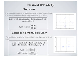
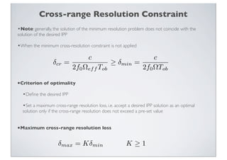
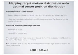
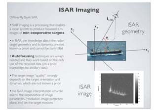
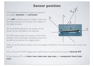
The document discusses optimal sensor positioning for ISAR imaging. It describes how the image projection plane (IPP) depends on the sensor position and target motion, and how obtaining certain desired IPPs like front, side or top views constrain the sensor position angles. It presents a signal model relating Doppler frequency to scatterer position and sensor angles. The constraints for different desired IPPs and for minimizing cross-range resolution are described. Numerical results map target motion distributions to optimal sensor position distributions based on measured boat motion data.

1. OPTIMAL SENSOR
POSITIONING FOR ISAR
IMAGING
Marco Martorella
IGARSS 2010
HONOLULU, HAWAII, JULY 2010

2. Motivation
•In ISAR, long data recordings are often needed in order to form
an image with desired characteristics (useful for target
classification)
•Such image characteristics depend of both the target motions
and the sensor position
•Since the target is often non-cooperative, only the sensor
position can be used as a degree of freedom to drive the outcome
towards the desired result
Need of a simple tool that provides the means for
predicting the optimal sensor position: this will
minimise the time on target and maximise the
probability of obtaining a desired image

3. Outline
•Background
•ISAR imaging
•Image Projection Plane (IPP)
•Sensor position as a degree of freedom
•Signal model
•IPP constraints
•Front, Side, Top and Composite target views
•Cross-range resolution constraint
•Numerical results
•Conslusions

4. ISAR Imaging
Differently from SAR, i LOS
•ISAR imaging is a processing that enables x3 ISAR
a radar system to produce focussed e.m. x2
images of non-cooperative targets geometry
θe
•In ISAR, the knowledge about the radar-
target geometry and its dynamics are not
known a priori and cannot be controlled θa
x1
•Autofocusing techniques are always
needed and they work based on the only
use of the received data (no a priori
knowledge, no ancillary data)
•The target image “quality” strongly
depends on the target orientation and
dynamics, which are not known a priori
ISAR
•the ISAR image interpretation is harder
due to the dependence of image image
parameters (resolution, image projection
plane, etc) on the target motions

5. Image Projection Plane (IPP)
•Effective rotation vector Ω
Ωeff = i LOS × ( Ω × i LOS )
i LOS
Ωeff
•Image projection plane
( icr , ir ) = ( iLOS × Ωeff , iLOS )
•The image projection plane is a plane orthogonal to the
effective rotation vector
•The image projection plane depends on the effective rotation vector
and the radar-target Line of Sight
•The target plays a role in this since its own motions strongly
contribute to the target’s rotation vector and hence to the effective
rotation vector
•The IPP becomes very important when dealing with ISAR image interpretation (target’s projection
onto the image plane), which can be seen as a first step towards target classification and recognition

6. Sensor position
i LOS
•The position of the sensor is given by means of
two angles: azimuth and elevation
x3
x2
•The IPP is defined once the target’s motion and
the relative position of the sensor with respect to θe
the target are given
•In some ISAR applications, the position of the θa x1
sensor can be controlled by the operator
•In ISAR system design, the position of the sensor
becomes one of the system parameters that has to
be defined to optimise the imaging system
•We can see the sensor position as the only degree of freedom if we want to have some control over
the IPP
•As a criterion for ISAR imaging system optimisation, we will use the concept of desired IPP
•Typical desired IPPs are: front view, side view, top view and composite front/side
view

7. Signal model (1)
Tob=1.5 s
=
Ideal Scatterers
RADAR
•The cross-range image formation can be seen as a Doppler analysis
•Scatterers in different position along the cross-range direction produce different Doppler and
therefore are mapped in different cross-range positions in the image
•The Doppler induced by a scatterer positioned at x can be calculated analytically
2
fd (t) = [Ωef f (t) × x]
λ

8. Signal model (2)
•The Doppler frequency can also be calculated by using a matrix notation
2 2 T
fd (t) = [Ωef f (t) × x] = Ω (t) Lx
λ λ
Scatterer’s position
Effective rotation vector Rotation vector
Sensor position
related matrix
•where L is a 3x3 matrix with elements equal to
L11 = L22 = L33 = 0
L12 = −L21 = sin θe
L31 = −L13 = cos θe sin θa
L23 = −L32 = cos θa cos θe
•The Doppler frequency can therefore be rewritten as the sum of three contributions
fd (t) = L1 (t) x1 + L2 (t) x2 + L3 (t) x3
where Li ( t ) i = 1, 2, 3 are the Doppler Generating Factors (DGF)
L1 (t) = Ω2 (t) L21 + Ω3 (t) L31
L2 (t) = Ω1 (t) L12 + Ω3 (t) L32
L3 (t) = Ω1 (t) L13 + Ω2 (t) L23

9. Desired IPP (1/4)
3D Target Composite
front/side view
Front view Side view Top view

10. Desired IPP (2/4)
•A desired IPP can be obtained by acting on the sensor position
•For front, side and top views, this can be done by constraining
•one DGF
•one of the two angles that define the sensor position
•For a composite front/side view, this can be done by constraining
•two DGFs
•none of the angles that define the sensor position

11. Desired IPP (3/4)
Front view
•The contribution relative to the coordinate x must be forced to zero
1
•The sensor must be located in the plane formed by x and x
2 3
L1 (t) = −Ω2 (t) sin θe + Ω3 (t) cos θe sin θa = 0
subject to θa = π 2
Ω3 (t)
θe (t) = arctan
Ω2 (t)
Side view
•The contribution relative to the coordinate x must be forced to zero
2
•The sensor must be located in the plane formed by x and x
1 3
L2 (t) = Ω1 (t) sin θe − Ω3 (t) cos θa cos θe = 0,
subject to θa = 0
Ω3 (t)
θe (t) = arctan
Ω1 (t)

12. Desired IPP (4/4)
Top view
•The contribution relative to the coordinate x must be forced to zero
3
•The sensor must be located in the plane formed by x and x 1 2
L3 (t) = −Ω1 (t) cos θe sin θa + Ω2 (t) cos θa cos θe = 0
subject to θe = 0
Ω2 (t)
θa (t) = arctan
Ω1 (t)
Composite front/side view
•The contribution relative to the coordinates x 1 and x2 must be forced
to zero
L1 (t) = −Ω2 (t) sin θe + Ω3 (t) cos θe sin θa = 0
L2 (t) = Ω1 (t) sin θe − Ω3 (t) cos θa cos θe = 0
Ω2 (t)
θa (t) = arctan Ω1 (t)
Ω3 (t)
θe (t) = arctan √
Ω1 (t)+Ω2 (t)

13. Cross-range Resolution Constraint
•The solution of the problem of obtaining a desired IPP may produce an image with poor cross-
range resolution
•The cross-range resolution can be determined in the case of constant target rotation vector
c
δcr =
2f0 Ωef f Tob Ωeff = i LOS × ( Ω × i LOS )
•Note: the effective rotation vector can be small even when the target rotation vector is large
because of a bad choice of the sensor position
•Given a target rotation vector, the sensor position that minimises
the cross-range resolution can
be obtained by constraining the inner product between the radar LoS and the target rotation
vector to zero
Ω · iLoS = cos θa cos θe Ω1 + sin θa cos θe Ω2 + sin θe Ω3 = 0
•There are an infinite number of solutions. The generic solution can be written as
Ω1 cos θa + Ω2 sin θa
θe = − arctan
Ω3

14. Cross-range Resolution Constraint
•Note: generally, the solution of the minimum resolution problem does not coincide with the
solution of the desired IPP
•When the minimum cross-resolution constraint is not applied
c c
δcr = ≥ δmin =
2f0 Ωef f Tob 2f0 ΩTob
•Criterion of optimality
•Define the desired IPP
•Set a maximum cross-range resolution loss, i.e. accept a desired IPP solution as an optimal
solution only if the cross-range resolution does not exceed a pre-set value
•Maximum cross-range resolution loss
δmax = Kδmin K≥1

15. Mapping target motion distribution onto
optimal sensor position distribution
Non-cooperative target motions
•are not known a priori and in a general case cannot be predicted with sufficient accuracy
•depend on several parameters: both internal (e.g. target’s maneuvers) and external (e.g. sea
conditions for a ship)
Statistical distribution of target motions
•derived from models
•derived from measurements
•For each target motion, there exist an optimal sensor position that can be determined by applying
the desired IPP and cross-resolution constaints
•We can see the result as a map that transforms elements from the target motion space onto the
sensor position space
fΩ ( ω ) → fΘ (θ a ,θ e )

16. Numerical results (1/3)
DATA SET
•Pitch, roll and yaw motions of a small boat have been measured by using an Inertial
Measurement Unit (IMU)
•3500 samples at a rate of 0.2 sample/s
Normalised histograms of Pitch, roll and yaw
Pitch rate Roll rate Yaw rate
0.16 0.25 0.2
0.18
0.14
0.2 0.16
0.12
0.14
0.1
0.15 0.12
Probability
Probability
Probability
0.08 0.1
0.1 0.08
0.06
0.06
0.04
0.05 0.04
0.02
0.02
0 0 0
8 6 4 2 0 2 4 6 20 15 10 5 0 5 10 15 20 6 4 2 0 2 4
Degrees/s Degrees/s Degrees/s
•We can interpret the histograms as approximation of Probability Density Functions

17. Numerical results (2/3)
Side View
L2 (t) = Ω1 (t) sin θe − Ω3 (t) cos θa cos θe = 0,
subject to θa = 0
K=3
Ω3 (t)
θe (t) = arctan
Ω1 (t)
Pitch rate
0.16
0.14
Histogram Elevation Effective pure side view a
= 0 degrees
0.12
0.2
0.1
Probability
0.08 0.18
0.06
0.16
0.04
0.14
0.02
0 0.12
probability
8 6 4 2 0 2 4 6
Degrees/s
Yaw rate 0.1
0.2
0.18
0.08
0.16
0.14 0.06
0.12
Probability
0.1
0.04
0.08
0.02
0.06
0.04 0
0.02
0 0.2 0.4 0.6 0.8 1 1.2 1.4 1.6
e
0
6 4 2 0 2 4
Degrees/s

18. Numerical results (3/3)
Composite Front/Side View
L1 (t) = −Ω2 (t) sin θe + Ω3 (t) cos θe sin θa = 0
L2 (t) = Ω1 (t) sin θe − Ω3 (t) cos θa cos θe = 0
K=3
Ω2 (t)
θa (t) = arctan Ω1 (t)
Ω3 (t)
θe (t) = arctan √
Ω1 (t)+Ω2 (t)
Pitch rate Roll rate
Probability of effective mixed front/side view
0.16 0.25 90
0.03
0.14
0.2
0.12
80
0.1
0.15
0.025
70
Probability
Probability
0.08
0.1
0.06
60 0.02
0.04
0.05
0.02 50
e
0
8 6 4 2 0 2 4 6
0
20 15 10 5 0 5 10 15 20
0.015
Degrees/s Degrees/s 40
Yaw rate
0.2
0.18 30 0.01
0.16
0.14 20
0.12 0.005
Probability
0.1 10
0.08
0.06
0
0.04 0 10 20 30 40 50 60 70 80 90
0.02 a
0
6 4 2 0 2 4
Degrees/s

19. Conclusions
•Definition of optimality criteria for ISAR sensor positioning
•Mathematical derivation of a tool for predicting the optimal
sensor position
•Useful for placement of static sensors given the surveillance
scenario
•Useful for route planning of moving sensors
•Useful for predicting the probability of obtaining a desired IPP
given a scenario of interest and the position of the sensor
•Can be extended to bistatic and multistatic scenarios (please
check the proceedings of next EURAD conference)