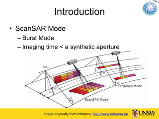
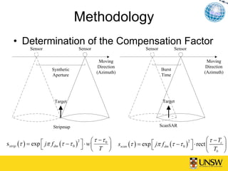
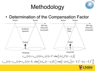
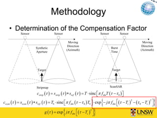
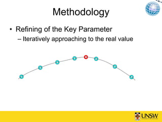
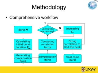
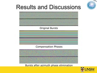
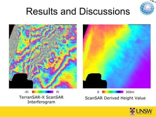
Blind Azimuth Phase
Elimination for TerraSAR-X
ScanSAR Interferometry
Alex Zhe Hu, Linlin Ge and Xiaojing Li
Geodesy and Earth Observing Systems Group (GEOS),
School of Surveying and Spatial Information Systems,
The University of New South Wales, Sydney, Australia
Email: z.hu@student.unsw.edu.au
Contents
•   Introduction
•   Methodology
•   Results and Discussions
•   Concluding Remarks
Contents
•   Introduction
•   Methodology
•   Results and Discussions
•   Concluding Remarks
Introduction
• ScanSAR Mode
 – Burst Mode
 – Imaging time < a synthetic aperture


                                                           Stripmap Mode


                                     ScanSAR Mode


          image originally from Infoterra: http://www.infoterra.de
Introduction
• ScanSAR Mode
 – Cover multiple swathes
 – Large range coverage


                                                           Stripmap Mode


                                     ScanSAR Mode


          image originally from Infoterra: http://www.infoterra.de
Introduction
• ScanSAR Interferometry
  – Cover multiple swathes
  – Large range coverage

  – Global DEM
  – Large-scale Earthquakes
Introduction
 • ScanSAR Interferometry
  ALOS          EnviSAT
                             RADARSAT TerraSAR-X
 PALSAR          ASAR
  L-band        C-band        C-band        X-band

250–350km        400km       300–500km      150km

   100m        75–150m        50–100m      up to 16m
                Ortiz and    Holzner and
Shimada 2007                                   ?
               Zebker 2007   Bamler 2002
Introduction
• TerraSAR-X ScanSAR Interferometry
  – Distortion and signal loss in azimuth direction
    after resampling
  – Only SLC data available for the public
Introduction
• TerraSAR-X ScanSAR Interferometry
  – Distortion and signal loss in azimuth direction
    after resampling
  – Only SLC data available for the public

  – Blind Azimuth Phase Elimination
Contents
•   Introduction
•   Methodology
•   Results and Discussions
•   Concluding Remarks
Methodology
• Phase Estimation Strategy


  – The simulated burst for compensation should
    have similar fringe patterns
Methodology
• Brief workflow
               Determination of the
               Compensation Factor


               Coarse Initialisation of
                the Key Parameter


                       Refining of
                   the Key Parameter


                     Elimination of
                   the Azimuth Phase
Methodology
   • Determination of the Compensation Factor
            Sensor                    Sensor                               Sensor           Sensor

                                                 Moving                                                    Moving
                                                 Direction                                                 Direction
                        Synthetic                                                   Burst
                                                (Azimuth)                                                 (Azimuth)
                        Aperture                                                    Time


                         Target                                                      Target


                        Stripmap                                                    ScanSAR


                                              ⎛ τ −τ 0 ⎞                                                    ⎛ τ − Tc ⎞
s strip (τ ) = exp ⎡ jπ f dm (τ − τ 0 ) ⎤ ⋅ w ⎜              sscan (τ ) = exp ⎡ jπ f dm (τ − τ 0 ) ⎤ ⋅ rect ⎜
                                       2                                                          2
                   ⎣                     ⎦ ⎝ T ⎟                              ⎣                     ⎦                ⎟
                                                       ⎠                                                    ⎝   Tb ⎠
Methodology
    • Determination of the Compensation Factor
             Sensor                   Sensor                                Sensor           Sensor

                                                 Moving                                                   Moving
                                                 Direction                                                Direction
                        Synthetic                                                    Burst
                                                (Azimuth)                                                (Azimuth)
                        Aperture                                                     Time


                          Target                                                      Target


                         Stripmap                                                    ScanSAR

                         cstrip (τ ) = sstrip (τ ) ∗ sref (τ ) = T ⋅ sinc ⎡π f dmT (τ − τ 0 ) ⎤
                                                                          ⎣                   ⎦

                                                ⎣                     ⎦     {
cscan (τ ) = sscan (τ ) ∗ sref (τ ) = Tb ⋅ sinc ⎡π f dm (τ − τ 0 ) Tb ⎤ ⋅ exp − jπ f dm ⎡(τ − Tc ) − (τ 0 − Tc ) ⎤
                                                                                        ⎣
                                                                                                  2             2
                                                                                                                  }
                                                                                                                  ⎦
Methodology
    • Determination of the Compensation Factor
             Sensor                   Sensor                                Sensor           Sensor

                                                    Moving                                                Moving
                                                    Direction                                             Direction
                        Synthetic                                                    Burst
                                                   (Azimuth)                                             (Azimuth)
                        Aperture                                                     Time


                          Target                                                      Target


                         Stripmap                                                    ScanSAR

                         cstrip (τ ) = sstrip (τ ) ∗ sref (τ ) = T ⋅ sinc ⎡π f dmT (τ − τ 0 ) ⎤
                                                                          ⎣                   ⎦

                                                ⎣                     ⎦     {
cscan (τ ) = sscan (τ ) ∗ sref (τ ) = Tb ⋅ sinc ⎡π f dm (τ − τ 0 ) Tb ⎤ ⋅ exp − jπ f dm ⎡(τ − Tc ) − (τ 0 − Tc ) ⎤
                                                                                        ⎣
                                                                                                  2             2
                                                                                                                  }
                                                                                                                  ⎦

                                               {
                               g (τ ) = exp jπ f dm ⎡(τ − Tc ) ⎤
                                                    ⎣
                                                              2
                                                                ⎦     }
Methodology
• Determination of the Compensation Factor
   Sensor                      Sensor                               Sensor           Sensor

                                         Moving                                                         Moving
                                         Direction                                                      Direction
                Synthetic                                                    Burst
                                        (Azimuth)                                                      (Azimuth)
                Aperture                                                     Time


                 Target                                                       Target


                Stripmap                                                     ScanSAR

                                              {
                               g (τ ) = exp jπ f dm ⎡(τ − Tc ) ⎤
                                                    ⎣
                                                              2
                                                                ⎦      }
   cscan (τ ) = ⎣ sscan (τ ) ∗ sref (τ ) ⎦ ⋅ g (τ ) = Tb ⋅ sinc ⎡π f dm (τ − τ 0 ) Tb ⎤ ⋅ exp ( jφ )
                ⎡                        ⎤                      ⎣                     ⎦
Methodology
• Coarse Initialisation of the Key Parameter
  g (τ ) = exp { jπ f dm ⎡(τ − Tc ) ⎤} = exp { jπ f dm ⎡(τ − Ts − Tb 2 ) ⎤}
                                   2                                    2
                         ⎣           ⎦                 ⎣                  ⎦
    – The compensation factor is a function of burst
      duration Tb
Methodology
• Coarse Initialisation of the Key Parameter
   cscan (τ ) = sscan (τ ) ∗ sref (τ ) = F −1 { F ⎡ sscan (τ ) ⎤ ⋅ F ⎡ sref (τ ) ⎤}
                                                  ⎣            ⎦ ⎣               ⎦
                       {  ⎣                      ⎦ ⎣               }
               = F −1 a ⋅ ⎡ S strip (ω ) ∗W (ω ) ⎤ ⋅ F ⎡ sref (τ ) ⎤
                                                                   ⎦


 1
aTb
           { {
    ⋅ F −1 F F ⎡cscan (τ ) ⎤ F ⎡ sref (τ ) ⎤
               ⎣           ⎦ ⎣             ⎦    }     ⎣              ⎦ }
                                                    F ⎡ S strip (ω ) ⎤ = sinc (Tbω )


    – time difference between two peaks of sinc
      function is determined by Tb
Methodology
• Coarse Initialisation of the Key Parameter
Methodology
• Refining of the Key Parameter
  – Iteratively approaching to the real value
Methodology
• Comprehensive workflow
                         Y

                       Correlation   N    Increasing
      Burst N
                       decreasing?            Tb


    Calculating        Computing             Fitting
    initial burst      correlation       correlation to
    duration Tb0         factor          find the peak


    Generating
                      compensation        Final comp
   compensation
                         Burst               Burst
      Burst
Contents
•   Introduction
•   Methodology
•   Results and Discussions
•   Concluding Remarks
Results and Discussions
  Information            Master Image                              Slave Image
Acquisition Date       16 February 2010                       27 February 2010
Acquisition Start
                       02:56:12 (UTC)                         02:56:13 (UTC)
     Time
Acquisition Stop
                       02:56:30 (UTC)                         02:56:31 (UTC)
     Time
   Number of
                                         4 (strip_04 – strip_07)
    Swathes
Number of Bursts    59 (strip_04 – strip_07)              61 (strip_04 – strip_07)
Central Latitude          28.785 °                                  28.785 °

Central Longitude         47.514 °                                   47.513°
Range Resolution         2.504 (metre)                             2.503 (metre)
    Azimuth
                         18.5 (metre)                              18.5 (metre)
   Resolution
Results and Discussions


        Original Bursts
Results and Discussions


        Original Bursts


      Compensation Phases
Results and Discussions


              Original Bursts


           Compensation Phases


   Bursts after azimuth phase elimination
Results and Discussions


Resampled slave   Burst-based interferogram
Results and Discussions


  -Pi          Pi          0            300m
TerranSAR-X ScanSAR   ScanSAR Derived Height Value
    Interferogram
Results and Discussions


      ScanSAR Derived DEM
Results and Discussions


      -50            50m
Height difference to SRTM DEM   Histogram of the difference
Contents
•   Introduction
•   Methodology
•   Results and Discussions
•   Concluding Remarks
Concluding Remarks
• Simplifying the TerraSAR-X ScanSAR
  interferometry by making it Stripmap-like
• Precise enough to remove the non-linear
  azimuth phases
• Providing a solution for TerraSAR-X
  ScanSAR interferometry starts from SLC
  data
• Can also be applied to other advanced
  SAR system with non-linear azimuth
  phases, such as Spotlight
Acknowledgement:

The authors are grateful to Infoterra for providing the
TerraSAR-X ScanSAR dataset on this research.

The first author also sincerely thanks GEOS and the Faculty of
Engineering of UNSW for supporting his scholarship on his PhD
study.

5_IGARSS2011_HU.pdf

  • 1.
    Blind Azimuth Phase Eliminationfor TerraSAR-X ScanSAR Interferometry Alex Zhe Hu, Linlin Ge and Xiaojing Li Geodesy and Earth Observing Systems Group (GEOS), School of Surveying and Spatial Information Systems, The University of New South Wales, Sydney, Australia Email: z.hu@student.unsw.edu.au
  • 2.
    Contents • Introduction • Methodology • Results and Discussions • Concluding Remarks
  • 3.
    Contents • Introduction • Methodology • Results and Discussions • Concluding Remarks
  • 4.
    Introduction • ScanSAR Mode – Burst Mode – Imaging time < a synthetic aperture Stripmap Mode ScanSAR Mode image originally from Infoterra: http://www.infoterra.de
  • 5.
    Introduction • ScanSAR Mode – Cover multiple swathes – Large range coverage Stripmap Mode ScanSAR Mode image originally from Infoterra: http://www.infoterra.de
  • 6.
    Introduction • ScanSAR Interferometry – Cover multiple swathes – Large range coverage – Global DEM – Large-scale Earthquakes
  • 7.
    Introduction • ScanSARInterferometry ALOS EnviSAT RADARSAT TerraSAR-X PALSAR ASAR L-band C-band C-band X-band 250–350km 400km 300–500km 150km 100m 75–150m 50–100m up to 16m Ortiz and Holzner and Shimada 2007 ? Zebker 2007 Bamler 2002
  • 8.
    Introduction • TerraSAR-X ScanSARInterferometry – Distortion and signal loss in azimuth direction after resampling – Only SLC data available for the public
  • 9.
    Introduction • TerraSAR-X ScanSARInterferometry – Distortion and signal loss in azimuth direction after resampling – Only SLC data available for the public – Blind Azimuth Phase Elimination
  • 10.
    Contents • Introduction • Methodology • Results and Discussions • Concluding Remarks
  • 11.
    Methodology • Phase EstimationStrategy – The simulated burst for compensation should have similar fringe patterns
  • 12.
    Methodology • Brief workflow Determination of the Compensation Factor Coarse Initialisation of the Key Parameter Refining of the Key Parameter Elimination of the Azimuth Phase
  • 13.
    Methodology • Determination of the Compensation Factor Sensor Sensor Sensor Sensor Moving Moving Direction Direction Synthetic Burst (Azimuth) (Azimuth) Aperture Time Target Target Stripmap ScanSAR ⎛ τ −τ 0 ⎞ ⎛ τ − Tc ⎞ s strip (τ ) = exp ⎡ jπ f dm (τ − τ 0 ) ⎤ ⋅ w ⎜ sscan (τ ) = exp ⎡ jπ f dm (τ − τ 0 ) ⎤ ⋅ rect ⎜ 2 2 ⎣ ⎦ ⎝ T ⎟ ⎣ ⎦ ⎟ ⎠ ⎝ Tb ⎠
  • 14.
    Methodology • Determination of the Compensation Factor Sensor Sensor Sensor Sensor Moving Moving Direction Direction Synthetic Burst (Azimuth) (Azimuth) Aperture Time Target Target Stripmap ScanSAR cstrip (τ ) = sstrip (τ ) ∗ sref (τ ) = T ⋅ sinc ⎡π f dmT (τ − τ 0 ) ⎤ ⎣ ⎦ ⎣ ⎦ { cscan (τ ) = sscan (τ ) ∗ sref (τ ) = Tb ⋅ sinc ⎡π f dm (τ − τ 0 ) Tb ⎤ ⋅ exp − jπ f dm ⎡(τ − Tc ) − (τ 0 − Tc ) ⎤ ⎣ 2 2 } ⎦
  • 15.
    Methodology • Determination of the Compensation Factor Sensor Sensor Sensor Sensor Moving Moving Direction Direction Synthetic Burst (Azimuth) (Azimuth) Aperture Time Target Target Stripmap ScanSAR cstrip (τ ) = sstrip (τ ) ∗ sref (τ ) = T ⋅ sinc ⎡π f dmT (τ − τ 0 ) ⎤ ⎣ ⎦ ⎣ ⎦ { cscan (τ ) = sscan (τ ) ∗ sref (τ ) = Tb ⋅ sinc ⎡π f dm (τ − τ 0 ) Tb ⎤ ⋅ exp − jπ f dm ⎡(τ − Tc ) − (τ 0 − Tc ) ⎤ ⎣ 2 2 } ⎦ { g (τ ) = exp jπ f dm ⎡(τ − Tc ) ⎤ ⎣ 2 ⎦ }
  • 16.
    Methodology • Determination ofthe Compensation Factor Sensor Sensor Sensor Sensor Moving Moving Direction Direction Synthetic Burst (Azimuth) (Azimuth) Aperture Time Target Target Stripmap ScanSAR { g (τ ) = exp jπ f dm ⎡(τ − Tc ) ⎤ ⎣ 2 ⎦ } cscan (τ ) = ⎣ sscan (τ ) ∗ sref (τ ) ⎦ ⋅ g (τ ) = Tb ⋅ sinc ⎡π f dm (τ − τ 0 ) Tb ⎤ ⋅ exp ( jφ ) ⎡ ⎤ ⎣ ⎦
  • 17.
    Methodology • Coarse Initialisationof the Key Parameter g (τ ) = exp { jπ f dm ⎡(τ − Tc ) ⎤} = exp { jπ f dm ⎡(τ − Ts − Tb 2 ) ⎤} 2 2 ⎣ ⎦ ⎣ ⎦ – The compensation factor is a function of burst duration Tb
  • 18.
    Methodology • Coarse Initialisationof the Key Parameter cscan (τ ) = sscan (τ ) ∗ sref (τ ) = F −1 { F ⎡ sscan (τ ) ⎤ ⋅ F ⎡ sref (τ ) ⎤} ⎣ ⎦ ⎣ ⎦ { ⎣ ⎦ ⎣ } = F −1 a ⋅ ⎡ S strip (ω ) ∗W (ω ) ⎤ ⋅ F ⎡ sref (τ ) ⎤ ⎦
  • 19.
    Methodology • Coarse Initialisationof the Key Parameter cscan (τ ) = sscan (τ ) ∗ sref (τ ) = F −1 { F ⎡ sscan (τ ) ⎤ ⋅ F ⎡ sref (τ ) ⎤} ⎣ ⎦ ⎣ ⎦ { ⎣ ⎦ ⎣ } = F −1 a ⋅ ⎡ S strip (ω ) ∗W (ω ) ⎤ ⋅ F ⎡ sref (τ ) ⎤ ⎦ 1 aTb { { ⋅ F −1 F F ⎡cscan (τ ) ⎤ F ⎡ sref (τ ) ⎤ ⎣ ⎦ ⎣ ⎦ } ⎣ ⎦ } F ⎡ S strip (ω ) ⎤ = sinc (Tbω ) – time difference between two peaks of sinc function is determined by Tb
  • 20.
  • 21.
    Methodology • Refining ofthe Key Parameter – Iteratively approaching to the real value
  • 22.
    Methodology • Comprehensive workflow Y Correlation N Increasing Burst N decreasing? Tb Calculating Computing Fitting initial burst correlation correlation to duration Tb0 factor find the peak Generating compensation Final comp compensation Burst Burst Burst
  • 23.
    Contents • Introduction • Methodology • Results and Discussions • Concluding Remarks
  • 24.
    Results and Discussions Information Master Image Slave Image Acquisition Date 16 February 2010 27 February 2010 Acquisition Start 02:56:12 (UTC) 02:56:13 (UTC) Time Acquisition Stop 02:56:30 (UTC) 02:56:31 (UTC) Time Number of 4 (strip_04 – strip_07) Swathes Number of Bursts 59 (strip_04 – strip_07) 61 (strip_04 – strip_07) Central Latitude 28.785 ° 28.785 ° Central Longitude 47.514 ° 47.513° Range Resolution 2.504 (metre) 2.503 (metre) Azimuth 18.5 (metre) 18.5 (metre) Resolution
  • 25.
    Results and Discussions Original Bursts
  • 26.
    Results and Discussions Original Bursts Compensation Phases
  • 27.
    Results and Discussions Original Bursts Compensation Phases Bursts after azimuth phase elimination
  • 28.
    Results and Discussions Resampledslave Burst-based interferogram
  • 29.
    Results and Discussions -Pi Pi 0 300m TerranSAR-X ScanSAR ScanSAR Derived Height Value Interferogram
  • 30.
    Results and Discussions ScanSAR Derived DEM
  • 31.
    Results and Discussions -50 50m Height difference to SRTM DEM Histogram of the difference
  • 32.
    Contents • Introduction • Methodology • Results and Discussions • Concluding Remarks
  • 33.
    Concluding Remarks • Simplifyingthe TerraSAR-X ScanSAR interferometry by making it Stripmap-like • Precise enough to remove the non-linear azimuth phases • Providing a solution for TerraSAR-X ScanSAR interferometry starts from SLC data • Can also be applied to other advanced SAR system with non-linear azimuth phases, such as Spotlight
  • 34.
    Acknowledgement: The authors aregrateful to Infoterra for providing the TerraSAR-X ScanSAR dataset on this research. The first author also sincerely thanks GEOS and the Faculty of Engineering of UNSW for supporting his scholarship on his PhD study.