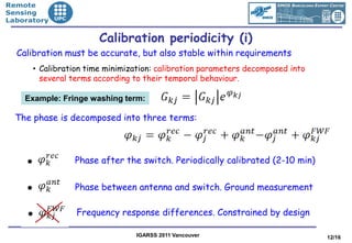
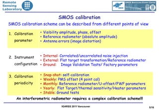
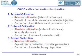
This document discusses calibration of the SMOS (Soil Moisture and Ocean Salinity) Earth Explorer mission. SMOS uses an interferometric radiometer called MIRAS to measure brightness temperatures. MIRAS requires comprehensive calibration to correct for measurement errors. The calibration scheme involves internal noise injection, external sky views by a reference radiometer, and ground characterization. The goal is to parameterize errors, measure coefficients, extract errors through calibration, and assess residuals to iteratively refine the error model.
![•Remote
•Sensing
•Laboratory
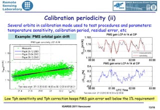
The error model (ii)
Residual error assessment and iterative fine tuning of the error model has
been a key approach to improve subsystem performance
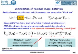
Example: digital correlator offset
With 1-0 correction With 1-0 and truncation error correction
0.6 0.6
Mean= -0.21-0.22i cu
0.4 0.4
σ=0.03cu
Mean= -0.00061+0.00029i cu
0.2 σ=0.029cu
0.2
ℑ m[M] (cu)
ℑ m[M] (cu)
0 0
-0.2 -0.2
-0.4 -0.4
avg~1min avg ~12h avg ~12h
-0.4 -0.2 0 0.2 0.4 0.6 -0.4 -0.2 0 0.2 0.4 0.6
ℜ e[M] (cu) ℜ e[M] (cu)
m≈10-3 m≈2·10-5 MIRAS:
m≈6·10-8
AMIRAS: MIRAS:
σ ≈10-4 σ ≈3·10-6 σ ≈3·10-6
IGARSS 2011 Vancouver 9/16](https://image.slidesharecdn.com/igarss11-end-to-end-calibration-v2-110728105437-phpapp02/85/IGARSS11-End-to-end-calibration-v2-pdf-9-320.jpg)
![•Remote
•Sensing
•Laboratory
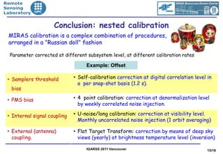
The error model (iv)
Correlation denormalization: PMS gain and correlator loss are measured in-
flight well within requirements: amplitude error < 1%
Correlator loss PMS gain error
5 0.5
4 0.4
0.3
RMS[%]
3
%
2 0.2
0.1
1
0
0 0 20 40 60
0 500 1000 1500 2000 2500 Receiver number
Test data start: 24-12-2009 00:44:39 to 25-12-200900:05:14
Baseline number
In-flight measured Correlation Loss ~1.5 % RMS gain error after Tph correction ~0.2 %
IGARSS 2011 Vancouver 11/16](https://image.slidesharecdn.com/igarss11-end-to-end-calibration-v2-110728105437-phpapp02/85/IGARSS11-End-to-end-calibration-v2-pdf-11-320.jpg)