The document contains lecture notes on algorithm design techniques, including greedy algorithms, divide and conquer, dynamic programming, approximation algorithms, and local search. It provides examples of problems that can be solved using each technique and outlines algorithms for interval scheduling, scheduling to minimize lateness, finding closest pair of points, weighted interval scheduling, and more. It also introduces matroids as a theoretical foundation for greedy algorithms and proves properties like maximum independent sets having the same size.
![Lecture Notes On
Algo-Design
Lecturer: Ulf-Peter Schroeder
February 16, 2006
written by:
Braun, Rudolf
Brune, Philipp
Piepmeyer, Meik
Please send corrections - including [AlgoDesign-Script] in the subject line -
to: meikp <KLAMMERAFFE> upb <PUNKT> de
1](https://image.slidesharecdn.com/script-mda1-101011070309-phpapp01/85/Script-md-a-1-1-320.jpg)
![Lecture Notes On
Algo-Design
Lecturer: Ulf-Peter Schroeder
February 16, 2006
written by:
Braun, Rudolf
Brune, Philipp
Piepmeyer, Meik
Please send corrections - including [AlgoDesign-Script] in the subject line -
to: meikp <KLAMMERAFFE> upb <PUNKT> de
1](https://image.slidesharecdn.com/script-mda1-101011070309-phpapp01/75/Script-md-a-1-1-2048.jpg)
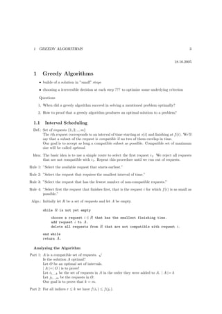
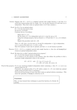
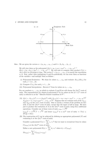
![1 GREEDY ALGORITHMS 4
Proof: r=1 Our Greedy Rule guaranties that f (i1 ) ≤ f (j1 ).
I.H.: The statement is true for r − 1.
I.S.: We know that f (jr−1 ) ≤ s(jr ). Combining this with the I.H: f (ir−1 ) ≤ f (jr−1 )
we get f (ir−1 ) ≤ s(jr ). Since interval jr is one of available interests at the time when the
greedy algorithm selects ir , we have f (ir ) ≤ f (jr ).
Part 3: The greedy algorithm returns an optimal set A.
Proof: ( given by contradiction )
If A is not optimal then an optimal set 0 must have more requests, that is, we must have
m > k. Applying Part 2 with r = k, then is f (ik ) ≤ f (jk ). Since m > k, there is a request
jk+1 in O.
This request starts after request jk ends, and ends after ik ends. But the greedy algorithm
stops with request ik , and it is only supposed to stop when R is empty. `
25.10.2005
1.2 Scheduling to Minimize Lateness
Definition of the Problem
A single ressource, a set of n requests to use the ressource for an interval of time, ressource is
available starting at time S, the request i has a deadline di , and it requires a continuous time
interval of length ti . Each request must be assigned non overlapping intervals.
Objective function
We will assign each request i an interval of time of length ti , let us denote this interval [s(i), f (i)]
with f (i) = s(i) + ti .
We say that a request i is late if it misses the deadline, that is if di < f (i).
li = f (i) − di . We say that li = 0 if request i is not late.
maximum lateness L = max li
i∈{1,..,n}
Idea 1: ”Schedule the jobs in order of increasing length ti .”
Idea 2: ”Schedule the jobs in order of increasing slacktime di − ti ”.
Idea 3: ”Earliest Deadline First”
Analyzing the ”Earliest Deadline First” - Greedy Algorithm
We start with an optimized schedule O.
Our plan we have is to gradually modify O, perserving its optimality at each step, but transforming
it into a schedule that is indicated to the schedule A formed by our algorithm.
Fact 1: There is an optimal schedule with no idle time.
Def.: A schedule A′ has an inversion if a job i with deadline di is scheduled before another job j
with earlier deadline dj < di .
Fact 2: All schedules with no inversions and no idle time have the same maximum lateness.
Fact 3: There is an optimal schedule that has no inversions and no idle time.
Proof of Fact 3: By Fact 1 there is an optimal schedule with no idle time.](https://image.slidesharecdn.com/script-mda1-101011070309-phpapp01/85/Script-md-a-1-4-320.jpg)
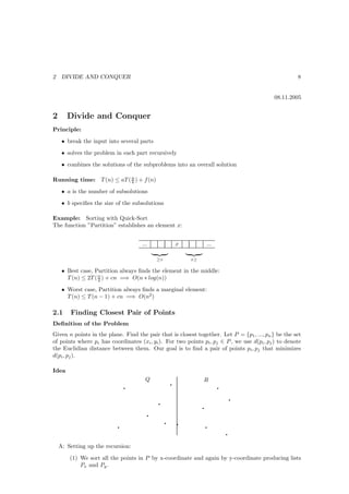
![1 GREEDY ALGORITHMS 5
1. If O has an inversion, then there is a pair of jobs i and j and that j is immediately
after i and has dj < di .
2. After swapping i and j, we get a schedule with one less inversion.
√
3. The new swapped schedule has a maximum lateness no longer then that of O.
Proof of (3.): All jobs other then jobs i and j finish at the same time in the two schedules.
˜i = f (i) − di = f (j) − di < f (j) − dj = l′
l ˜
j
⇐⇒ ˜i < lj
l ′
Notation
Optimal schedule O: each request r is scheduled [s(r), f (r)]
′
and has lateness lr
L′ = max lr
′
r
swapped schedule O : s(r), f (r), ˜r , L
˜ ˜ ˜ l ˜
1.3 ( Huffman Codes and Data Compressions )
1.4 Theoretical foundations for the greedy method
Def.: A matroid is a pair M = (S, I) satisfying the following conditions:
1. S is a finite non-empty set
1
2. I is a non-empty family of subsets of S such that: B ∈ I and A ⊂ B implies A ∈ I.
3. If A ∈ I, B ∈ I and |A| < |B|, then there exists some element x ∈ B A such that
A ∪ [x] ∈ I. 2
Examples: 1. Matrix Matroid
Def.: S = set of n-vectors
I consists of all subsets of linear independent vectors from S.
1 1 1 0
A = 0 0 1 1
1 0 1 1
1
1 1 0
S = 0, 0, 1, 1
1
0 1 1
e1 e2 e3 e4
I = {∅, {e1 }, {e2}, {e3 }, {e4 }, {e1 , e2 }, {e1, e3 }, {e1 , e4 }, {e2 , e3 }, {e2, e4 },
{e3 , e4 }, {e1, e2 , e3 }, {e1 , e2 , e4 }, {e1, e3 , e4 }}
2. Graphic Matroid
Def.: Let G = (V, E) be a continued, undirected graph.
MG = (SG , IG ) is defined by SG = E. I consists of all subset A ⊂ E such that
(V, A) is acyclic.
1 hereditary
2 exchange property](https://image.slidesharecdn.com/script-mda1-101011070309-phpapp01/85/Script-md-a-1-5-320.jpg)
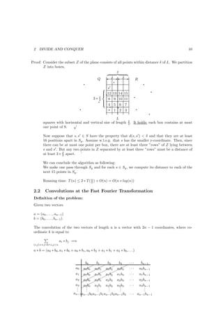
![1 GREEDY ALGORITHMS 6
1. and 2. trivial.
3. exchange property?
Let A and B belong to I with |A| < |B|, i.e. A and B are forests. Let V (A), V (B)
be sets of vertices incident to edges from A and B, resp.
(a) If b ∈ V (B) V (A), then exists some e ∈ V (B) such that [b, e] ∈ B.
A ∪ {(b, c)} is acyclic.
(b) Now we can assume that V (B) ⊂ V (A)
( Theorem: Forest with k edges contains exactly |V | − k trees. )
A consists of τ1 = |V (A)| − |A| trees and
B consists of τ2 = |V (B)| − |B| trees.
|V (B)| ≤ |V (A)| and |A| < |B| implies τ2 < τ1 .
=⇒ ∃ some edge e ∈ B connecting 2 trees from A
=⇒ A ∪ {e} is acyclic.
3. ”counter example”
Interval Scheduling
S = {1, .., n} be the set of requests.
U ⊂ S belongs to I if its requests are mutually compatible.
Def.: Let M = [S, I] be a matroid.
A ∈ I is called maximal, if there exists no x ∈ S A such that A ∪ {x} ∈ I.
Lemma: All maximum independent subsets in a matroid have the same size.
Proof: Suppose the contrary:
There exist two maximum independent subsets A, B with |A| < |B|.
` to the exchange property.
3
Example: 1. A is maximal ⇔ |A| = rank(S)
4
2. A is maximal ⇔ A is spanning tree of G ⇔ |A| = |V | − 1
Def.: A Matroid M = (S, I) is called weighted if there is a weight w(x) > 0 to each x ∈ S.
For A ⊂ S we set w(A) = x⊂A w(x).
The maximum weight independent subset problem: Find a maximum weight independent
subset in a weighted matroid.
Greedy(M,w)
A=∅
sort S[M ] into nonincreasing order by weight w
for each x ∈ S[M ] take in nonincreasing order by weight w do
if A ∪ {x} ∈ I(M ) then
A := A ∪ {x}
return A
MST: Define the matroid MG = (SG , IG ) with SG = E. IS consists of all subsets A ⊂ E such that
(V, A) is acyclic.
We define w′ (e) = (wmax + 1) − w(e) with wmax = max{w(e)}.
e∈E
It holds w′ (e) > 0 ∀e ∈ E and Greedy(MI , w′ ) computes an optimal subset5 which is a MST
in the original graph.
3 rank means rank for the Matrix Matroid.
4 |V | means vertices for the Graphire Matroid.
5 that means a maximum weight independent subset](https://image.slidesharecdn.com/script-mda1-101011070309-phpapp01/85/Script-md-a-1-6-320.jpg)

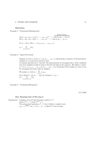
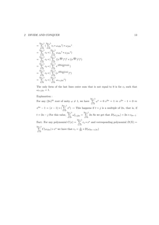
![3 DYNAMIC PROGRAMMING 15
OP T (6)
OP T (5) OP T (3)
OP T (4) OP T (3) OP T (2) OP T (1)
OP T (3) OP T (0) OP T (2) OP T (1) OP T (1) OP T (0)
OP T (2) OP T (1) OP T (1) OP T (0)
OP T (1) OP T (0)
Example:
Remark 2: A fundamental observation, which forms the second crucial component of a dynamic pro-
gramming solution, is that our recursive algorithm is really only solving n + 1 different sub
solutions.
How could we eliminate the redundancy?
=⇒ ”Memorization”
22.11.2005
”Memorization”
M [0..n]: M [j] will start with the value ”empty” but will hold the value of OP T (j) as soon as it is
first determined.
M-OPT(j)
if j=0 then
return 0
else
if M[j] is not empty then
return M[j]
else
M[j] = max(vj + M-OPT(p(j)), M-OPT(j − 1))
return M[j]
Iterative-M-OPT(j)](https://image.slidesharecdn.com/script-mda1-101011070309-phpapp01/85/Script-md-a-1-15-320.jpg)
![3 DYNAMIC PROGRAMMING 16
M[0] = 0
for j=1,..,n
M[j] = max(vj + M − (p(j)), M (j − 1))
return M[j]
So far we have simply computed the value of an optimal solution. What we want is the full
optimal set of intervals as well. We know from Fact 2 that j belongs to an optimal solution for
the set of intervals {1, .., j} iff 6 vj + OP T (p(j)) ≥ OP T (j − 1).
Find Solution(j)
if j=0 then
Output nothing
else
if vj + M [p(j)] ≥ M [j − 1] then
Output j together with the result of Find Solution(p(j))
else
Output the result of Find Solution(j-1)
”Informal Guidelines”
1. There are only a polynomial number of subproblems
2. The solution to the original problem can be easily computed from the solutions to the
subproblems.
3. There is a natural ordering on subproblems from ”smallest” to ”largest” together with an
easy to compute recurrence that allows one to determine the solution to a subproblem from
the solutions to some number of smaller subproblems
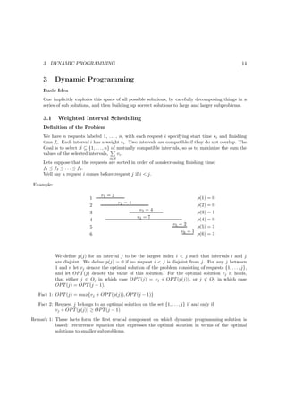
3.2 Segmented Least Squares
y
T
r
d
d d
rd
d dr
d
r
d d
d
dr
r
d d
d
dr
E
x
6 ”iff” means ”if and only if”](https://image.slidesharecdn.com/script-mda1-101011070309-phpapp01/85/Script-md-a-1-16-320.jpg)
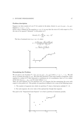
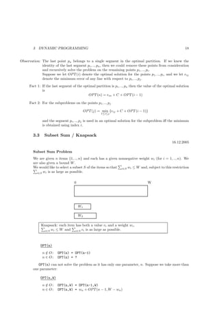
![3 DYNAMIC PROGRAMMING 19
OPT(i,W) = max{OP T (i − 1, W ), wi + OP T (i − 1, W − wi )}
SubsetSum(n, W)
Array M[0..n,0..W]
Initialize M[0,w] = 0 ∀w ∈ {0, .., w}
For i=1 to n
For j=0 to w
compute M[i,j] = max{M [i − 1, j], wi + M [i − 1, j − vi ]}
return M[m,W]
n
i
i-1
.
.
.
1
0
0 1 2 ... j ... W
Fact 1: The SubsetSum(n, W) Algorithm correctly computes the optimal value if the problem and
runs in O(n ∗ W ) time.
Note 1: The running time is a polynomial function of n and W , the largest integer involved in defining
the problem. We call such algorithms ”pseudo-polynomial”.
Extension to the Knapsack problem
n ∈ O:
/ OPT(n,W) = OPT(n-1,W)
n ∈ O: OPT(n,W) = wn + OP T (n − 1, W − wn )
Fact 2: If w < vi , then OP T (i, W ) = OP T (i − 1, W )
else n ∈ O: OPT(i,W) = max{OP T (i − 1, W ), vi + OP T (i − 1, W − wi )}
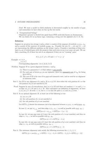
3.4 Sequence Alignment
Motivation
1. ”Online dictionaries”
Input: o c c u r r a n c e
Output: Do you mean o c c u r r e n c e ?
o currance o curr ance
occurrence occurre nce
costmism + costgap < 3 ∗ costgap ?](https://image.slidesharecdn.com/script-mda1-101011070309-phpapp01/85/Script-md-a-1-19-320.jpg)

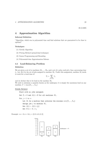
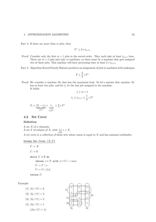


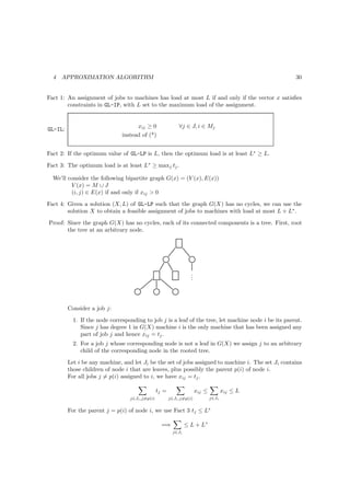
![4 APPROXIMATION ALGORITHM 32
The algorithm will run in polynomial time for any fixed choice ǫ 0 however, the dependence
on ǫ will not be polynomial. We call such an algorithm a “Polynomial-time approximation
scheme” (PTAS).
We already know an dynamic programming algorithm that run in O(n · W ).
“Old”: OP T (i, W )
“New”: OP T (i, V ) is the smallest knapsack weight W so that one can obtain a solution using a
subset of items 1, ..., i with values at least V .
i
We will have a subproblem for all i = 0, ..., n and values V = 0, ..., vj .
j=1
i
vj ≤ n · (max vi ) = n · v ∗ ⇒ O(n2 · v ∗ ) subproblems.
j=1 i
v∗
Recurrence for solving these subproblems:
n−1
if V vi then OP T (n, V ) = wn + OP T (n − 1, V − vn )
i=1
else OP T (n, V ) = min{OP T (n − 1, v), wn + OP T (n − 1, max(0, V − vn ))}
Knapsack (n)
Array M [0...n, 0...v]
For i = 0...n do M [i, 0] = 0
For i = 1, ..., n do
i
For v = 1, ..., vj do
j=1
i−1
if v vj then
j=1
M [i, v] = wi + M [i − 1, v]
else
M [i, v] = minM [i − 1, v], wi + M [i − 1, max0, v − vi ]
return the maximum value V such that M [n, V ] ≤ W
Idea for a PTAS:
If the values are small integers, then v ∗ is small and the problem can be solved in polynomial
time already. On the other hand, we will use a rounding parameter b and will consider the values
rounded to an integer multiple of b. More precisely, for each item i, let its rounded value be
vi = vi · b.
˜ b
We will use our dynamic programming algorithm to solve the problem with the rounded values.
Fact 1: For each item i we have vi ≤ vi ≤ vi + b. The rounded values are all integers multiples of a
˜
common value b. Instead of solving the problem with the rounded values vi , we can change
˜
˜
the units; we can divide all values by b and get an equivalent problem. vi = vi = vi for
ˆ b b
all i = 1, ..., n .](https://image.slidesharecdn.com/script-mda1-101011070309-phpapp01/85/Script-md-a-1-32-320.jpg)

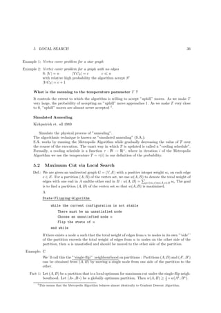
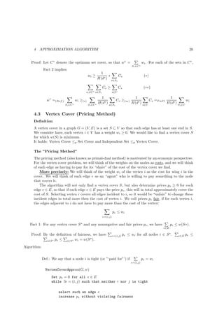
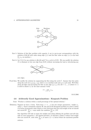
![5 LOCAL SEARCH 37
Proof : Let W = e∈E we . For two nodes u and v, we use wuv to denote we if there is an edge
e joining u and v and 0 otherwise. After the termination of the algorithm it holds for any
node u ∈ A
v∈A wuv ≤ v∈B wuv
We add up this inequalities for all u ∈ A :
2∗ (u,v)⊆A wuv ≤ u∈A,v∈B wuv = w(A, B) (*)
We can apply the same reasoning for B :
2∗ (u,v)⊆B wuv ≤ u∈A,v∈B wuv = w(A, B) (**)
⇒2∗( (u,v)⊆A wuv + (u,v)⊆B wuv ) ≤ 2 ∗ u∈A,v∈B wuv [add * and **]
⇒( (u,v)⊆A wuv + (u,v)⊆B wuv ) ≤ u∈A,v∈B wuv
⇒ w(A, B) + ( (u,v)⊆A wuv + (u,v)⊆B wuv ) ≤ 2 ∗ w(A, B)
⇒ w ≤ 2 ∗ w(A, B)
For the global optimal partition (A∗ , B ∗ ) we have w(A∗ , B ∗ ) ≤ W
⇒ w(A∗ , B ∗ ) ≤ 2 ∗ w(A, B)
Fact 2: The Single-Flip-Algorithm is pseudo-polynomial ( It is an open problem whether a local
optimum can be found in polynomial time).
Def.: Let (A, B) be a partition with weight w(A, B). For a fixed ǫ 0, let us say that a single-flip
of a node is a big-improvement-flip if it improves the cut value by at least 2∗ǫ ∗ w(A, B)
n
where n = |V |. Now consider a version of the single-flip-algorithm where we only accept
bit-improvement-flips and terminate once such a flip doesn’t exist.
Fact 3: Let (A, B) be a partition such that no big-improvement-flip is possible. Let (A∗ , B ∗ ) be a
globally optimal partition. Then (w + ǫ) ∗ w(A, B) ≥ w(A∗ , B ∗ )
Proof:
Fact 4: The version of the single-flip-algorithm that only accepts big-improvement-flips terminates
after at most O(ǫ−1 ∗ n ∗ logW ) flips, assuming the weights are integral and W = e∈E we .
Proof: Each flip improves the objective function by at least a factor of (1 + n ). [w(A, B) + 2∗ǫ ∗
ǫ
n
2∗ǫ 1 x
w(A, B) = w(A, B) ∗ (1 + n )] Since (1 + x ) ≥ 2 for any x ≥ 1 we get with x = n ≥ 1.
ǫ
ǫ ǫ
(1 + n ) n ≥ 2. This means that the objective function increases by a factor of at least 2
every n flips. The weight cannot exceed W , and hence it can be doubled at most log2 W
ǫ
times ⇒ O( n ∗ logW ) flips.
ǫ
5.3 Local search Algorithms for Graph-Partitioning
state-flipping-algorithm
Neighbour relations is the single-flip-rule.
k-flip-neighbourhood for k ≥ 1
We say that partitions (A, B) and (A′ , B ′ ) are neighbours under the k-flip rule if (A′ , B ′ ) can be
obtained from (A, B) by moving at most k nodes from one side of a partition to the other.](https://image.slidesharecdn.com/script-mda1-101011070309-phpapp01/85/Script-md-a-1-37-320.jpg)
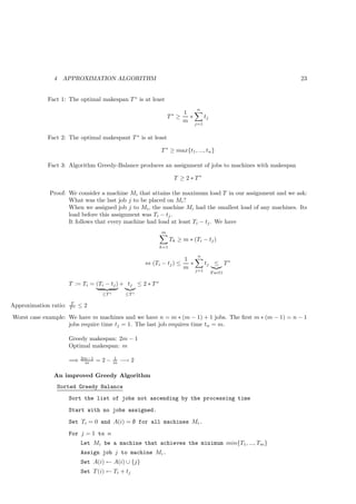
![5 LOCAL SEARCH 38
Kernigham, Lin ( 1970) ( KL-heuristic]
KL-heuristic defines the neighbours of a partition (A, B) according to the following n-phase pro-
cedure
• In phase 1, we choose a single-node-flip in such way that the value of the resulting solution is
as large as possible. We perform this flip even if the value of the solution decreases the value
of w(A, B). We mark the node that has been flipped. [Let (A1 , B1 ) denote the resulting
solution].
• At the start of phase k, for k 1, we have a partition (Ak−1 , Bk−1 ) and k − 1 nodes are
marked. We choose a single unmarked node to flip, in such a way that the resulting solution
is as large as possible. [Let (Ak , Bk ) denote the resulting solution and mark the node we
flip.]
After n phases : (An , Bn ) is the mirror image of the original partition (A, B), i.e. An =
B, Bn = A.
• We define n − 1 partitions (A1 , B1 ) . . . (An−1 , Bn−1 ) to be neighbours of (A, B). Thus (A, B)
is a local optimum under the KL-heuristic if and only if w(A, B) w(Ai , Bi ) for 1 ≤ i ≤ n−1.
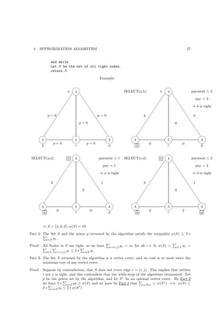
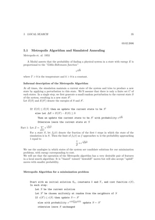
5.4 Best Response Dynamics and Nash-Equilibria
Definition:
We have a directed graph G = (V, E) with a cost ce ≥ 0 on each edge. There is a designated source
node s ∈ V and a collection of k agents located at distinct terminal nodes t1 , t2 , . . . tk ∈ V . Each
agent tj wants to construct a path Pj from s to tj using as little total cost as possible. Suppose
that after all the agents have chosen their paths, agent tj only needs to pay its ”‘fair share”’ of
the cost of each edge e on the path. That is, rather than paying ce for each e on Pj , it pays only
ce divided by the number of agents whose paths contain e.
Example:
Best response dynamics Each agent was continually prepared to improve its solution in response to changes made by
the other agents.
Nash-Equilibrium Stable solutions, where the best response of each agent is to stay fix. No agent has an
incentive to deviate.
Social Optimum It is the solution where it minimise the total cost to all agents.](https://image.slidesharecdn.com/script-mda1-101011070309-phpapp01/85/Script-md-a-1-38-320.jpg)