SlideShare a Scribd company logo
1 of 63
Download to read offline
Introduction to Numerical 
Methods 
Lecture notes for MATH 3311 
Jeffrey R. Chasnov 
The Hong Kong University of 
Science and Technology
The Hong Kong University of Science and Technology 
Department of Mathematics 
Clear Water Bay, Kowloon 
Hong Kong 
Copyright ○c 2012 by Jeffrey Robert Chasnov 
This work is licensed under the Creative Commons Attribution 3.0 Hong Kong License. 
To view a copy of this license, visit http://creativecommons.org/licenses/by/3.0/hk/ 
or send a letter to Creative Commons, 171 Second Street, Suite 300, San Francisco, 
California, 94105, USA.
Preface 
What follows are my lecture notes for Math 3311: Introduction to Numerical 
Methods, taught at the Hong Kong University of Science and Technology. Math 
3311, with two lecture hours per week, is primarily for non-mathematics majors 
and is required by several engineering departments. 
All web surfers are welcome to download these notes at 
http://www.math.ust.hk/~machas/numerical-methods.pdf 
and to use the notes freely for teaching and learning. I welcome any comments, 
suggestions or corrections sent by email to jeffrey.chasnov@ust.hk. 
iii
Contents 
1 IEEE Arithmetic 1 
1.1 Definitions . . . . . . . . . . . . . . . . . . . . . . . . . . . . . . . 1 
1.2 Numbers with a decimal or binary point . . . . . . . . . . . . . . 1 
1.3 Examples of binary numbers . . . . . . . . . . . . . . . . . . . . . 1 
1.4 Hex numbers . . . . . . . . . . . . . . . . . . . . . . . . . . . . . 1 
1.5 4-bit unsigned integers as hex numbers . . . . . . . . . . . . . . . 2 
1.6 IEEE single precision format: . . . . . . . . . . . . . . . . . . . . 2 
1.7 Special numbers . . . . . . . . . . . . . . . . . . . . . . . . . . . 3 
1.8 Examples of computer numbers . . . . . . . . . . . . . . . . . . . 3 
1.9 Inexact numbers . . . . . . . . . . . . . . . . . . . . . . . . . . . 4 
1.9.1 Find smallest positive integer that is not exact in single 
precision . . . . . . . . . . . . . . . . . . . . . . . . . . . . 4 
1.10 Machine epsilon . . . . . . . . . . . . . . . . . . . . . . . . . . . . 5 
1.11 IEEE double precision format . . . . . . . . . . . . . . . . . . . . 5 
1.12 Roundoff error example . . . . . . . . . . . . . . . . . . . . . . . 6 
2 Root Finding 7 
2.1 Bisection Method . . . . . . . . . . . . . . . . . . . . . . . . . . . 7 
2.2 Newton’s Method . . . . . . . . . . . . . . . . . . . . . . . . . . . 7 
2.3 Secant Method . . . . . . . . . . . . . . . . . . . . . . . . . . . . 8 
2.3.1 Estimate 
√ 
2 = 1.41421356 using Newton’s Method . . . . 8 
2.3.2 Example of fractals using Newton’s Method . . . . . . . . 8 
2.4 Order of convergence . . . . . . . . . . . . . . . . . . . . . . . . . 9 
2.4.1 Newton’s Method . . . . . . . . . . . . . . . . . . . . . . . 9 
2.4.2 Secant Method . . . . . . . . . . . . . . . . . . . . . . . . 10 
3 Systems of equations 13 
3.1 Gaussian Elimination . . . . . . . . . . . . . . . . . . . . . . . . . 13 
3.2 퐿푈 decomposition . . . . . . . . . . . . . . . . . . . . . . . . . . 14 
3.3 Partial pivoting . . . . . . . . . . . . . . . . . . . . . . . . . . . . 17 
3.4 Operation counts . . . . . . . . . . . . . . . . . . . . . . . . . . . 18 
3.5 System of nonlinear equations . . . . . . . . . . . . . . . . . . . . 21 
4 Least-squares approximation 23 
4.1 Fitting a straight line . . . . . . . . . . . . . . . . . . . . . . . . 23 
4.2 Fitting to a linear combination of functions . . . . . . . . . . . . 24 
v
vi CONTENTS 
5 Interpolation 27 
5.1 Polynomial interpolation . . . . . . . . . . . . . . . . . . . . . . . 27 
5.1.1 Vandermonde polynomial . . . . . . . . . . . . . . . . . . 27 
5.1.2 Lagrange polynomial . . . . . . . . . . . . . . . . . . . . . 28 
5.1.3 Newton polynomial . . . . . . . . . . . . . . . . . . . . . . 28 
5.2 Piecewise linear interpolation . . . . . . . . . . . . . . . . . . . . 29 
5.3 Cubic spline interpolation . . . . . . . . . . . . . . . . . . . . . . 30 
5.4 Multidimensional interpolation . . . . . . . . . . . . . . . . . . . 33 
6 Integration 35 
6.1 Elementary formulas . . . . . . . . . . . . . . . . . . . . . . . . . 35 
6.1.1 Midpoint rule . . . . . . . . . . . . . . . . . . . . . . . . . 35 
6.1.2 Trapezoidal rule . . . . . . . . . . . . . . . . . . . . . . . 36 
6.1.3 Simpson’s rule . . . . . . . . . . . . . . . . . . . . . . . . 37 
6.2 Composite rules . . . . . . . . . . . . . . . . . . . . . . . . . . . . 37 
6.2.1 Trapezoidal rule . . . . . . . . . . . . . . . . . . . . . . . 37 
6.2.2 Simpson’s rule . . . . . . . . . . . . . . . . . . . . . . . . 38 
6.3 Local versus global error . . . . . . . . . . . . . . . . . . . . . . . 38 
6.4 Adaptive integration . . . . . . . . . . . . . . . . . . . . . . . . . 39 
7 Ordinary differential equations 43 
7.1 Examples of analytical solutions . . . . . . . . . . . . . . . . . . 43 
7.1.1 Initial value problem . . . . . . . . . . . . . . . . . . . . . 43 
7.1.2 Boundary value problems . . . . . . . . . . . . . . . . . . 44 
7.1.3 Eigenvalue problem . . . . . . . . . . . . . . . . . . . . . 45 
7.2 Numerical methods: initial value problem . . . . . . . . . . . . . 46 
7.2.1 Euler method . . . . . . . . . . . . . . . . . . . . . . . . . 46 
7.2.2 Modified Euler method . . . . . . . . . . . . . . . . . . . 46 
7.2.3 Second-order Runge-Kutta methods . . . . . . . . . . . . 47 
7.2.4 Higher-order Runge-Kutta methods . . . . . . . . . . . . 48 
7.2.5 Adaptive Runge-Kutta Methods . . . . . . . . . . . . . . 49 
7.2.6 System of differential equations . . . . . . . . . . . . . . . 50 
7.3 Numerical methods: boundary value problem . . . . . . . . . . . 51 
7.3.1 Finite difference method . . . . . . . . . . . . . . . . . . . 51 
7.3.2 Shooting method . . . . . . . . . . . . . . . . . . . . . . . 53 
7.4 Numerical methods: eigenvalue problem . . . . . . . . . . . . . . 54 
7.4.1 Finite difference method . . . . . . . . . . . . . . . . . . . 54 
7.4.2 Shooting method . . . . . . . . . . . . . . . . . . . . . . . 56
Chapter 1 
IEEE Arithmetic 
1.1 Definitions 
Bit = 0 or 1 
Byte = 8 bits 
Word = Reals: 4 bytes (single precision) 
8 bytes (double precision) 
= Integers: 1, 2, 4, or 8 byte signed 
1, 2, 4, or 8 byte unsigned 
1.2 Numbers with a decimal or binary point 
    ·     Decimal: 103 102 101 100 10−1 10−2 10−3 10−4 
Binary: 23 22 21 20 2−1 2−2 2−3 2−4 
1.3 Examples of binary numbers 
Decimal Binary 
1 1 
2 10 
3 11 
4 100 
0.5 0.1 
1.5 1.1 
1.4 Hex numbers 
{0, 1, 2, 3, . . . , 9, 10, 11, 12, 13, 14, 15} = {0, 1, 2, 3.......9, a,b,c,d,e,f} 
1
2 CHAPTER 1. IEEE ARITHMETIC 
1.5 4-bit unsigned integers as hex numbers 
Decimal Binary Hex 
1 0001 1 
2 0010 2 
3 0011 3 
... 
... 
... 
10 1010 a 
... 
... 
... 
15 1111 f 
1.6 IEEE single precision format: 
⏞ 푠⏟ 
0 
⏞ 푒⏟ 
1 
2 
3 
4 
5 
6 
78 
⏞ 푓⏟ 
9 
· · · · · · · ·31 
# = (−1)푠 × 2푒−127 × 1.f 
where s = sign 
e = biased exponent 
p=e-127 = exponent 
1.f = significand (use binary point)
1.7. SPECIAL NUMBERS 3 
1.7 Special numbers 
Smallest exponent: e = 0000 0000, represents denormal numbers (1.f → 0.f) 
Largest exponent: e = 1111 1111, represents ±∞, if f = 0 
e = 1111 1111, represents NaN, if f̸= 0 
Number Range: e = 1111 1111 = 28 - 1 = 255 reserved 
e = 0000 0000 = 0 reserved 
so, p = e - 127 is 
1 - 127 ≤ p ≤ 254-127 
-126 ≤ p ≤ 127 
Smallest positive normal number 
= 1.0000 0000 · · · · ·· 0000× 2−126 
≃ 1.2 × 10−38 
bin: 0000 0000 1000 0000 0000 0000 0000 0000 
hex: 00800000 
MATLAB: realmin(’single’) 
Largest positive number 
= 1.1111 1111 · · · · ·· 1111× 2127 
= (1 + (1 − 2−23)) × 2127 
≃ 2128 ≃ 3.4 × 1038 
bin: 0111 1111 0111 1111 1111 1111 1111 1111 
hex: 7f7fffff 
MATLAB: realmax(’single’) 
Zero 
bin: 0000 0000 0000 0000 0000 0000 0000 0000 
hex: 00000000 
Subnormal numbers 
Allow 1.f → 0.f (in software) 
Smallest positive number = 0.0000 0000 · · · · · 0001 × 2−126 
= 2−23 × 2−126 ≃ 1.4 × 10−45 
1.8 Examples of computer numbers 
What is 1.0, 2.0  1/2 in hex ? 
1.0 = (−1)0 × 2(127−127) × 1.0 
Therefore, 푠 = 0, 푒 = 0111 1111, 푓 = 0000 0000 0000 0000 0000 000 
bin: 0011 1111 1000 0000 0000 0000 0000 0000 
hex: 3f80 0000 
2.0 = (−1)0 × 2(128−127) × 1.0 
Therefore, 푠 = 0, 푒 = 1000 0000, 푓 = 0000 0000 0000 0000 0000 000 
bin: 0100 00000 1000 0000 0000 0000 0000 0000 
hex: 4000 0000
4 CHAPTER 1. IEEE ARITHMETIC 
1/2 = (−1)0 × 2(126−127) × 1.0 
Therefore, 푠 = 0, 푒 = 0111 1110, 푓 = 0000 0000 0000 0000 0000 000 
bin: 0011 1111 0000 0000 0000 0000 0000 0000 
hex: 3f00 0000 
1.9 Inexact numbers 
Example: 
1 
3 
= (−1)0 × 
1 
4 
× (1 + 
1 
3 
), 
so that 푝 = 푒 − 127 = −2 and 푒 = 125 = 128 − 3, or in binary, 푒 = 0111 1101. 
How is 푓 = 1/3 represented in binary? To compute binary number, multiply 
successively by 2 as follows: 
0.333 . . . 0. 
0.666 . . . 0.0 
1.333 . . . 0.01 
0.666 . . . 0.010 
1.333 . . . 0.0101 
etc. 
so that 1/3 exactly in binary is 0.010101 . . . . With only 23 bits to represent 푓, 
the number is inexact and we have 
푓 = 01010101010101010101011, 
where we have rounded to the nearest binary number (here, rounded up). The 
machine number 1/3 is then represented as 
00111110101010101010101010101011 
or in hex 
3푒푎푎푎푎푎푏. 
1.9.1 Find smallest positive integer that is not exact in 
single precision 
Let 푁 be the smallest positive integer that is not exact. Now, I claim that 
푁 − 2 = 223 × 1.11 . . . 1, 
and 
푁 − 1 = 224 × 1.00 . . . 0. 
The integer 푁 would then require a one-bit in the 2−24 position, which is not 
available. Therefore, the smallest positive integer that is not exact is 224 + 1 = 
16 777 217. In MATLAB, single(224) has the same value as single(224+1). Since 
single(224+1) is exactly halfway between the two consecutive machine numbers 
224 and 224+2, MATLAB rounds to the number with a final zero-bit in f, which 
is 224.
1.10. MACHINE EPSILON 5 
1.10 Machine epsilon 
Machine epsilon (휖mach) is the distance between 1 and the next largest number. 
If 0 ≤ 훿  휖mach/2, then 1 + 훿 = 1 in computer math. Also since 
푥 + 푦 = 푥(1 + 푦/푥), 
if 0 ≤ 푦/푥  휖mach/2, then 푥 + 푦 = 푥 in computer math. 
Find 휖mach 
The number 1 in the IEEE format is written as 
1 = 20 × 1.000 . . . 0, 
with 23 0’s following the binary point. The number just larger than 1 has a 1 
in the 23rd position after the decimal point. Therefore, 
휖mach = 2−23 ≈ 1.192 × 10⁻⁷. 
What is the distance between 1 and the number just smaller than 1? Here, 
the number just smaller than one can be written as 
2−1 × 1.111 . . . 1 = 2−1(1 + (1 − 2−23)) = 1 − 2−24 
Therefore, this distance is 2−24 = 휖mach/2. 
The spacing between numbers is uniform between powers of 2, with logarith-mic 
spacing of the powers of 2. That is, the spacing of numbers between 1 and 
2 is 2−23, between 2 and 4 is 2−22, between 4 and 8 is 2−21, etc. This spacing 
changes for denormal numbers, where the spacing is uniform all the way down 
to zero. 
Find the machine number just greater than 5 
A rough estimate would be 5(1+휖mach) = 5+5휖mach, but this is not exact. The 
exact answer can be found by writing 
5 = 22(1 + 
1 
4 
), 
so that the next largest number is 
22(1 + 
1 
4 
+ 2−23) = 5 + 2−21 = 5 + 4휖mach. 
1.11 IEEE double precision format 
Most computations take place in double precision, where round-off error is re-duced, 
and all of the above calculations in single precision can be repeated for 
double precision. The format is 
⏞ 푠⏟ 
0 
⏞ 푒⏟ 
12 
3 
4 
5 
6 
7 
8 
9 
1011 
⏞ 푓⏟ 
12 
· · · · · · · ·63
6 CHAPTER 1. IEEE ARITHMETIC 
# = (−1)푠 × 2푒−1023 × 1.f 
where s = sign 
e = biased exponent 
p=e-1023 = exponent 
1.f = significand (use binary point) 
1.12 Roundoff error example 
Consider solving the quadratic equation 
푥2 + 2푏푥 − 1 = 0, 
where 푏 is a parameter. The quadratic formula yields the two solutions 
푥± = −푏 ± 
√︀ 
푏2 + 1. 
Consider the solution with 푏  0 and 푥  0 (the 푥+ solution) given by 
푥 = −푏 + 
√︀ 
푏2 + 1. (1.1) 
As 푏 → ∞, 
푥 = −푏 + 
√︀ 
푏2 + 1 
√︀ 
= −푏 + 푏 
1 + 1/푏2 
√︀ 
= 푏( 
1 + 1/푏2 − 1) 
≈ 푏 
(︂ 
1 + 
1 
2푏2 
− 1 
)︂ 
= 
1 
2푏 
. 
Now in double precision, realmin ≈ 2.2 × 10−308 and we would like 푥 to be 
accurate to this value before it goes to 0 via denormal numbers. Therefore, 
푥 should be computed accurately to 푏 ≈ 1/(2 × realmin) ≈ 2 × 10307. What 
happens if we compute (1.1) directly? Then 2 √ 
푥 = 0 when 푏+ 1 = 푏2, or 
1 + 1/푏2 = 1. That is 1/푏2 = 휖mach/2, or 푏 = 
2/ 
√ 
휖mach ≈ 108. 
For a subroutine written to compute the solution of a quadratic for a general 
user, this is not good enough. The way for a software designer to solve this 
problem is to compute the solution for 푥 as 
푥 = 
1 
푏 + 
√ 
푏2 + 1 
. 
In this form, if 푏2 +1 = 푏2, then 푥 = 1/2푏 which is the correct asymptotic form.
Chapter 2 
Root Finding 
Solve 푓(푥) = 0 for 푥, when an explicit analytical solution is impossible. 
2.1 Bisection Method 
The bisection method is the easiest to numerically implement and almost always 
works. The main disadvantage is that convergence is slow. If the bisection 
method results in a computer program that runs too slow, then other faster 
methods may be chosen; otherwise it is a good choice of method. 
We want to construct a sequence 푥0, 푥1, 푥2, . . . that converges to the root 
푥 = 푟 that solves 푓(푥) = 0. We choose 푥0 and 푥1 such that 푥0  푟  푥1. We 
say that 푥0 and 푥1 bracket the root. With 푓(푟) = 0, we want 푓(푥0) and 푓(푥1) 
to be of opposite sign, so that 푓(푥0)푓(푥1)  0. We then assign 푥2 to be the 
midpoint of 푥0 and 푥1, that is 푥2 = (푥0 + 푥1)/2, or 
푥2 = 푥0 + 
푥1 − 푥0 
2 
. 
The sign of 푓(푥2) can then be determined. The value of 푥3 is then chosen as 
either the midpoint of 푥0 and 푥2 or as the midpoint of 푥2 and 푥1, depending on 
whether 푥0 and 푥2 bracket the root, or 푥2 and 푥1 bracket the root. The root, 
therefore, stays bracketed at all times. The algorithm proceeds in this fashion 
and is typically stopped when the increment to the left side of the bracket 
(above, given by (푥1 − 푥0)/2) is smaller than some required precision. 
2.2 Newton’s Method 
This is the fastest method, but requires analytical computation of the derivative 
of 푓(푥). Also, the method may not always converge to the desired root. 
We can derive Newton’s Method graphically, or by a Taylor series. We again 
want to construct a sequence 푥0, 푥1, 푥2, . . . that converges to the root 푥 = 푟. 
Consider the 푥푛+1 member of this sequence, and Taylor series expand 푓(푥푛+1) 
about the point 푥푛. We have 
푓(푥푛+1) = 푓(푥푛) + (푥푛+1 − 푥푛)푓′(푥푛) + . . . . 
7
8 CHAPTER 2. ROOT FINDING 
To determine 푥푛+1, we drop the higher-order terms in the Taylor series, and 
assume 푓(푥푛+1) = 0. Solving for 푥푛+1, we have 
푥푛+1 = 푥푛 − 
푓(푥푛) 
푓′(푥푛) 
. 
Starting Newton’s Method requires a guess for 푥0, hopefully close to the root 
푥 = 푟. 
2.3 Secant Method 
The Secant Method is second best to Newton’s Method, and is used when a 
faster convergence than Bisection is desired, but it is too difficult or impossible 
to take an analytical derivative of the function 푓(푥). We write in place of 푓′(푥푛), 
푓′(푥푛) ≈ 
푓(푥푛) − 푓(푥푛−1) 
푥푛 − 푥푛−1 
. 
Starting the Secant Method requires a guess for both 푥0 and 푥1. 
2.3.1 Estimate 
√ 
2 = 1.41421356 using Newton’s Method 
The 
√ 
2 is the zero of the function 푓(푥) = 푥2 − 2. To implement Newton’s 
Method, we use 푓′(푥) = 2푥. Therefore, Newton’s Method is the iteration 
푥푛+1 = 푥푛 − 
푥2 
푛 − 2 
2푥푛 
. 
We take as our initial guess 푥0 = 1. Then 
푥1 = 1 − 
−1 
2 
= 
3 
2 
= 1.5, 
푥2 = 
3 
2 
− 
9 
4 − 2 
3 
= 
17 
12 
= 1.416667, 
푥3 = 
17 
12 
− 
172 
122 − 2 
17 
6 
= 
577 
408 
= 1.41426. 
2.3.2 Example of fractals using Newton’s Method 
Consider the complex roots of the equation 푓(푧) = 0, where 
푓(푧) = 푧3 − 1. 
These roots are the three cubic roots of unity. With 
푒푖2휋푛 = 1, 푛 = 0, 1, 2, . . . 
the three unique cubic roots of unity are given by 
1, 푒푖2휋/3, 푒푖4휋/3. 
With 
푒푖휃 = cos 휃 + 푖 sin 휃,
2.4. ORDER OF CONVERGENCE 9 
and cos (2휋/3) = −1/2, sin (2휋/3) = 
√ 
3/2, the three cubic roots of unity are 
푟1 = 1, 푟2 = − 
1 
2 
+ 
√ 
3 
2 
푖, 푟3 = − 
1 
2 
− 
√ 
3 
2 
푖. 
The interesting idea here is to determine which initial values of 푧0 in the complex 
plane converge to which of the three cubic roots of unity. 
Newton’s method is 
푧푛+1 = 푧푛 − 
푧3푛 
− 1 
3푧2푛 
. 
If the iteration converges to 푟1, we color 푧0 red; 푟2, blue; 푟3, green. The result 
will be shown in lecture. 
2.4 Order of convergence 
Let 푟 be the root and 푥푛 be the 푛th approximation to the root. Define the error 
as 
휖푛 = 푟 − 푥푛. 
If for large 푛 we have the approximate relationship 
|휖푛+1| = 푘|휖푛|푝, 
with 푘 a positive constant, then we say the root-finding numerical method is of 
order 푝. Larger values of 푝 correspond to faster convergence to the root. The 
order of convergence of bisection is one: the error is reduced by approximately 
a factor of 2 with each iteration so that 
|휖푛+1| = 
1 
2 
|휖푛|. 
We now find the order of convergence for Newton’s Method and for the Secant 
Method. 
2.4.1 Newton’s Method 
We start with Newton’s Method 
푥푛+1 = 푥푛 − 
푓(푥푛) 
푓′(푥푛) 
. 
Subtracting both sides from 푟, we have 
푟 − 푥푛+1 = 푟 − 푥푛 + 
푓(푥푛) 
푓′(푥푛) 
, 
or 
휖푛+1 = 휖푛 + 
푓(푥푛) 
푓′(푥푛) 
. (2.1)
10 CHAPTER 2. ROOT FINDING 
We use Taylor series to expand the functions 푓(푥푛) and 푓′(푥푛) about the root 
푟, using 푓(푟) = 0. We have 
푓(푥푛) = 푓(푟) + (푥푛 − 푟)푓′(푟) + 
1 
2 
(푥푛 − 푟)2푓′′(푟) + . . . , 
= −휖푛푓′(푟) + 
1 
2 
휖2 
푛푓′′(푟) + . . . ; 
푓′(푥푛) = 푓′(푟) + (푥푛 − 푟)푓′′(푟) + 
1 
2 
(푥푛 − 푟)2푓′′′(푟) + . . . , 
= 푓′(푟) − 휖푛푓′′(푟) + 
1 
2 
휖2 
푛푓′′′(푟) + . . . . 
(2.2) 
To make further progress, we will make use of the following standard Taylor 
series: 
1 
1 − 휖 
= 1 + 휖 + 휖2 + . . . , (2.3) 
which converges for |휖|  1. Substituting (2.2) into (2.1), and using (2.3) yields 
휖푛+1 = 휖푛 + 
푓(푥푛) 
푓′(푥푛) 
= 휖푛 + 
−휖푛푓′(푟) + 1 
2 휖2 
푛푓′′(푟) + . . . 
푓′(푟) − 휖푛푓′′(푟) + 1 
2 휖2 
푛푓′′′(푟) + . . . 
= 휖푛 + 
−휖푛 + 1 
2 휖2 
푛 
푓′′(푟) 
푓′(푟) + . . . 
1 − 휖푛 
푓′′(푟) 
푓′(푟) + . . . 
= 휖푛 + 
(︂ 
−휖푛 + 
1 
2 
휖2 
푛 
푓′′(푟) 
푓′(푟) 
+ . . . 
)︂(︂ 
1 + 휖푛 
푓′′(푟) 
푓′(푟) 
+ . . . 
)︂ 
= 휖푛 + 
(︂ 
−휖푛 + 휖2 
푛 
(︂ 
1 
2 
푓′′(푟) 
푓′(푟) 
− 
푓′′(푟) 
푓′(푟) 
)︂ 
+ . . . 
)︂ 
= − 
1 
2 
푓′′(푟) 
푓′(푟) 
휖2 
푛 + . . . 
Therefore, we have shown that 
|휖푛+1| = 푘|휖푛|2 
as 푛 → ∞, with 
푘 = 
1 
2 
⃒⃒⃒⃒ 
푓′′(푟) 
푓′(푟) 
⃒⃒⃒⃒ 
, 
provided 푓′(푟)̸= 0. Newton’s method is thus of order 2 at simple roots. 
2.4.2 Secant Method 
Determining the order of the Secant Method proceeds in a similar fashion. We 
start with 
푥푛+1 = 푥푛 − 
(푥푛 − 푥푛−1)푓(푥푛) 
푓(푥푛) − 푓(푥푛−1) 
. 
We subtract both sides from 푟 and make use of 
푥푛 − 푥푛−1 = (푟 − 푥푛−1) − (푟 − 푥푛) 
= 휖푛−1 − 휖푛,
2.4. ORDER OF CONVERGENCE 11 
and the Taylor series 
푓(푥푛) = −휖푛푓′(푟) + 
1 
2 
휖2 
푛푓′′(푟) + . . . , 
푓(푥푛−1) = −휖푛−1푓′(푟) + 
1 
2 
휖2 
푛−1푓′′(푟) + . . . , 
so that 
푓(푥푛) − 푓(푥푛−1) = (휖푛−1 − 휖푛)푓′(푟) + 
1 
2 
(휖2 
푛 − 휖2 
푛−1)푓′′(푟) + . . . 
= (휖푛−1 − 휖푛) 
(︂ 
푓′(푟) − 
1 
2 
(휖푛−1 + 휖푛)푓′′(푟) + . . . 
)︂ 
. 
We therefore have 
휖푛+1 = 휖푛 + 
−휖푛푓′(푟) + 1 
2 휖2 
푛푓′′(푟) + . . . 
푓′(푟) − 1 
2 (휖푛−1 + 휖푛)푓′′(푟) + . . . 
= 휖푛 − 휖푛 
1 − 1 
2 휖푛 
푓′′(푟) 
푓′(푟) + . . . 
2 (휖푛−1 + 휖푛) 푓′′(푟) 
푓′(푟) + . . . 
1 − 1 
= 휖푛 − 휖푛 
(︂ 
1 − 
1 
2 
휖푛 
푓′′(푟) 
푓′(푟) 
+ . . . 
)︂(︂ 
1 + 
1 
2 
(휖푛−1 + 휖푛) 
푓′′(푟) 
푓′(푟) 
+ . . . 
)︂ 
= − 
1 
2 
푓′′(푟) 
푓′(푟) 
휖푛−1휖푛 + . . . , 
or to leading order 
|휖푛+1| = 
1 
2 
⃒⃒⃒⃒ 
푓′′(푟) 
푓′(푟) 
⃒⃒⃒⃒ 
|휖푛−1||휖푛|. (2.4) 
The order of convergence is not yet obvious from this equation, and to determine 
the scaling law we look for a solution of the form 
|휖푛+1| = 푘|휖푛|푝. 
From this ansatz, we also have 
|휖푛| = 푘|휖푛−1|푝, 
and therefore 
|휖푛+1| = 푘푝+1|휖푛−1|푝2 
. 
Substitution into (2.4) results in 
푘푝+1|휖푛−1|푝2 
= 
푘 
2 
⃒⃒⃒⃒ 
푓′′(푟) 
푓′(푟) 
⃒⃒⃒⃒ 
|휖푛−1|푝+1. 
Equating the coefficient and the power of 휖푛−1 results in 
푘푝 = 
1 
2 
⃒⃒⃒⃒ 
푓′′(푟) 
푓′(푟) 
⃒⃒⃒⃒ 
, 
and 
푝2 = 푝 + 1.
12 CHAPTER 2. ROOT FINDING 
The order of convergence of the Secant Method, given by 푝, therefore is deter-mined 
to be the positive root of the quadratic equation 푝2 − 푝 − 1 = 0, or 
푝 = 
√ 
5 
2 
1 + 
≈ 1.618, 
which coincidentally is a famous irrational number that is called The Golden 
Ratio, and goes by the symbol Φ. We see that the Secant Method has an order 
of convergence lying between the Bisection Method and Newton’s Method.
Chapter 3 
Systems of equations 
Consider the system of 푛 linear equations and 푛 unknowns, given by 
푎11푥1 + 푎12푥2 + · · · + 푎1푛푥푛 = 푏1, 
푎21푥1 + 푎22푥2 + · · · + 푎2푛푥푛 = 푏2, 
... 
... 
푎푛1푥1 + 푎푛2푥2 + · · · + 푎푛푛푥푛 = 푏푛. 
We can write this system as the matrix equation 
Ax = b, 
with 
A = 
⎛ 
⎜⎜⎜⎝ 
푎11 푎12 · · · 푎1푛 
푎21 푎22 · · · 푎2푛 
... 
... 
. . . 
... 
푎푛1 푎푛2 · · · 푎푛푛 
⎞ 
⎟⎟⎟⎠ 
, x = 
⎛ 
⎜⎜⎜⎝ 
푥1 
푥2 
... 
푥푛 
⎞ 
⎟⎟⎟⎠ 
, b = 
⎛ 
⎜⎜⎜⎝ 
푏1 
푏2 
... 
푏푛 
⎞ 
⎟⎟⎟⎠ 
. 
3.1 Gaussian Elimination 
The standard numerical algorithm to solve a system of linear equations is called 
Gaussian Elimination. We can illustrate this algorithm by example. 
Consider the system of equations 
−3푥1 + 2푥2 − 푥3 = −1, 
6푥1 − 6푥2 + 7푥3 = −7, 
3푥1 − 4푥2 + 4푥3 = −6. 
To perform Gaussian elimination, we form an Augmented Matrix by combining 
the matrix A with the column vector b: 
⎛ 
⎝ 
⎞ 
⎠. 
−3 2 −1 −1 
6 −6 7 −7 
3 −4 4 −6 
Row reduction is then performed on this matrix. Allowed operations are (1) 
multiply any row by a constant, (2) add multiple of one row to another row, (3) 
13
14 CHAPTER 3. SYSTEMS OF EQUATIONS 
interchange the order of any rows. The goal is to convert the original matrix 
into an upper-triangular matrix. 
We start with the first row of the matrix and work our way down as follows. 
First we multiply the first row by 2 and add it to the second row, and add the 
first row to the third row: 
⎛ 
⎝ 
−3 2 −1 −1 
0 −2 5 −9 
0 −2 3 −7 
⎞ 
⎠. 
We then go to the second row. We multiply this row by −1 and add it to the 
third row: ⎛ 
−3 2 −1 −1 
0 −2 5 −9 
0 0 −2 2 
⎝ 
⎞ 
⎠. 
The resulting equations can be determined from the matrix and are given by 
−3푥1 + 2푥2 − 푥3 = −1 
−2푥2 + 5푥3 = −9 
−2푥3 = 2. 
These equations can be solved by backward substitution, starting from the last 
equation and working backwards. We have 
−2푥3 = 2 → 푥3 = −1 
−2푥2 = −9 − 5푥3 = −4 → 푥2 = 2, 
−3푥1 = −1 − 2푥2 + 푥3 = −6 → 푥1 = 2. 
Therefore, ⎛ 
푥1 
푥2 
푥3 
⎝ 
⎞ 
⎠ = 
⎛ 
⎝ 
⎞ 
⎠. 
2 
2 
−1 
3.2 퐿푈 decomposition 
The process of Gaussian Elimination also results in the factoring of the matrix 
A to 
A = LU, 
where L is a lower triangular matrix and U is an upper triangular matrix. 
Using the same matrix A as in the last section, we show how this factorization 
is realized. We have 
⎛ 
⎝ 
⎞ 
⎠ → 
−3 2 −1 
6 −6 7 
3 −4 4 
⎛ 
⎝ 
−3 2 −1 
0 −2 5 
0 −2 3 
⎞ 
⎠ = M1A, 
where 
M1A = 
⎛ 
⎝ 
⎞ 
⎠ 
1 0 0 
2 1 0 
1 0 1 
⎛ 
⎝ 
⎞ 
⎠ = 
−3 2 −1 
6 −6 7 
3 −4 4 
⎛ 
⎝ 
⎞ 
⎠. 
−3 2 −1 
0 −2 5 
0 −2 3
3.2. 퐿푈 DECOMPOSITION 15 
Note that the matrix M1 performs row elimination on the first column. Two 
times the first row is added to the second row and one times the first row is 
added to the third row. The entries of the column of M1 come from 2 = −(6/−3) 
and 1 = −(3/−3) as required for row elimination. The number −3 is called the 
pivot. 
The next step is 
⎛ 
⎝ 
⎞ 
⎠ → 
−3 2 −1 
0 −2 5 
0 −2 3 
⎛ 
⎝ 
⎞ 
⎠ = M2(M1A), 
−3 2 −1 
0 −2 5 
0 0 −2 
where 
M2(M1A) = 
⎛ 
⎝ 
⎞ 
⎠ 
1 0 0 
0 1 0 
0 −1 1 
⎛ 
⎝ 
⎞ 
⎠ = 
−3 2 −1 
0 −2 5 
0 −2 3 
⎛ 
⎝ 
⎞ 
⎠. 
−3 2 −1 
0 −2 5 
0 0 −2 
Here, M2 multiplies the second row by −1 = −(−2/ − 2) and adds it to the 
third row. The pivot is −2. 
We now have 
M2M1A = U 
or 
A = M−1 
1 M−1 
2 U. 
The inverse matrices are easy to find. The matrix M1 multiples the first row by 
2 and adds it to the second row, and multiplies the first row by 1 and adds it 
to the third row. To invert these operations, we need to multiply the first row 
by −2 and add it to the second row, and multiply the first row by −1 and add 
it to the third row. To check, with 
M1M−1 
1 = I, 
we have ⎛ 
⎝ 
⎞ 
⎠ 
1 0 0 
2 1 0 
1 0 1 
⎛ 
⎝ 
⎞ 
⎠ = 
1 0 0 
−2 1 0 
−1 0 1 
⎛ 
⎝ 
1 0 0 
0 1 0 
0 0 1 
⎞ 
⎠. 
Similarly, 
M−1 
2 = 
⎛ 
⎝ 
1 0 0 
0 1 0 
0 1 1 
⎞ 
⎠ 
Therefore, 
L = M−1 
1 M−1 
2 
is given by 
L = 
⎛ 
⎝ 
⎞ 
⎠ 
1 0 0 
−2 1 0 
−1 0 1 
⎛ 
⎝ 
⎞ 
⎠ = 
1 0 0 
0 1 0 
0 1 1 
⎛ 
⎝ 
⎞ 
⎠, 
1 0 0 
−2 1 0 
−1 1 1 
which is lower triangular. The off-diagonal elements of M−1 
1 and M−1 
2 are simply 
combined to form L. Our LU decomposition is therefore 
⎛ 
⎝ 
−3 2 −1 
6 −6 7 
3 −4 4 
⎞ 
⎠ = 
⎛ 
⎝ 
⎞ 
⎠ 
1 0 0 
−2 1 0 
−1 1 1 
⎛ 
⎝ 
⎞ 
⎠. 
−3 2 −1 
0 −2 5 
0 0 −2
16 CHAPTER 3. SYSTEMS OF EQUATIONS 
Another nice feature of the LU decomposition is that it can be done by over-writing 
A, therefore saving memory if the matrix A is very large. 
The LU decomposition is useful when one needs to solve Ax = b for x when 
A is fixed and there are many different b’s. First one determines L and U using 
Gaussian elimination. Then one writes 
(LU)x = L(Ux) = b. 
We let 
y = Ux, 
and first solve 
Ly = b 
for y by forward substitution. We then solve 
Ux = y 
for x by backward substitution. When we count operations, we will see that 
solving (LU)x = b is significantly faster once L and U are in hand than solving 
Ax = b directly by Gaussian elimination. 
We now illustrate the solution of LUx = b using our previous example, 
where 
L = 
⎛ 
⎝ 
⎞ 
⎠, U = 
1 0 0 
−2 1 0 
−1 1 1 
⎛ 
⎝ 
⎞ 
⎠, b = 
−3 2 −1 
0 −2 5 
0 0 −2 
⎛ 
⎝ 
−1 
−7 
−6 
⎞ 
⎠. 
With y = Ux, we first solve Ly = b, that is 
⎛ 
⎝ 
⎞ 
⎠ 
1 0 0 
−2 1 0 
−1 1 1 
⎛ 
⎝ 
푦1 
푦2 
푦3 
⎞ 
⎠ = 
⎛ 
⎝ 
⎞ 
⎠. 
−1 
−7 
−6 
Using forward substitution 
푦1 = −1, 
푦2 = −7 + 2푦1 = −9, 
푦3 = −6 + 푦1 − 푦2 = 2. 
We now solve Ux = y, that is 
⎛ 
⎝ 
⎞ 
⎠ 
−3 2 −1 
0 −2 5 
0 0 −2 
⎛ 
⎝ 
푥1 
푥2 
푥3 
⎞ 
⎠ = 
⎛ 
⎝ 
−1 
−9 
2 
⎞ 
⎠. 
Using backward substitution, 
−2푥3 = 2 → 푥3 = −1, 
−2푥2 = −9 − 5푥3 = −4 → 푥2 = 2, 
−3푥1 = −1 − 2푥2 + 푥3 = −6 → 푥1 = 2, 
and we have once again determined 
⎛ 
⎝ 
푥1 
푥2 
푥3 
⎞ 
⎠ = 
⎛ 
⎝ 
⎞ 
⎠. 
2 
2 
−1
3.3. PARTIAL PIVOTING 17 
3.3 Partial pivoting 
When performing Gaussian elimination, the diagonal element that one uses 
during the elimination procedure is called the pivot. To obtain the correct 
multiple, one uses the pivot as the divisor to the elements below the pivot. 
Gaussian elimination in this form will fail if the pivot is zero. In this situation, 
a row interchange must be performed. 
Even if the pivot is not identically zero, a small value can result in big round-off 
errors. For very large matrices, one can easily lose all accuracy in the solution. 
To avoid these round-off errors arising from small pivots, row interchanges are 
made, and this technique is called partial pivoting (partial pivoting is in contrast 
to complete pivoting, where both rows and columns are interchanged). We will 
illustrate by example the LU decomposition using partial pivoting. 
Consider 
A = 
⎛ 
⎝ 
⎞ 
⎠. 
−2 2 −1 
6 −6 7 
3 −8 4 
We interchange rows to place the largest element (in absolute value) in the pivot, 
or 푎11, position. That is, 
A → 
⎛ 
⎝ 
⎞ 
⎠ = P12A, 
6 −6 7 
−2 2 −1 
3 −8 4 
where 
P12 = 
⎛ 
⎝ 
0 1 0 
1 0 0 
0 0 1 
⎞ 
⎠ 
is a permutation matrix that when multiplied on the left interchanges the first 
and second rows of a matrix. Note that P−1 
12 = P12. The elimination step is 
then 
P12A → 
⎛ 
⎝ 
6 −6 7 
0 0 4/3 
0 −5 1/2 
⎞ 
⎠ = M1P12A, 
where 
M1 = 
⎛ 
⎝ 
⎞ 
⎠. 
1 0 0 
1/3 1 0 
−1/2 0 1 
The final step requires one more row interchange: 
M1P12A → 
⎛ 
⎝ 
⎞ 
⎠ = P23M1P12A = U. 
6 −6 7 
0 −5 1/2 
0 0 4/3 
Since the permutation matrices given by P are their own inverses, we can write 
our result as 
(P23M1P23)P23P12A = U.
18 CHAPTER 3. SYSTEMS OF EQUATIONS 
Multiplication of M on the left by P interchanges rows while multiplication on 
the right by P interchanges columns. That is, 
P23 
⎛ 
⎝ 
⎞ 
⎠P23 = 
1 0 0 
1/3 1 0 
−1/2 0 1 
⎛ 
⎝ 
1 0 0 
−1/2 0 1 
1/3 1 0 
⎞ 
⎠P23 = 
⎛ 
⎝ 
⎞ 
⎠. 
1 0 0 
−1/2 1 0 
1/3 0 1 
The net result on M1 is an interchange of the nondiagonal elements 1/3 and 
−1/2. 
We can then multiply by the inverse of (P23M1P23) to obtain 
P23P12A = (P23M1P23)−1U, 
which we write as 
PA = LU. 
Instead of L, MATLAB will write this as 
A = (P−1L)U. 
For convenience, we will just denote (P−1L) by L, but by L here we mean a 
permutated lower triangular matrix. 
For example, in MATLAB, to solve Ax = b for x using Gaussian elimination, 
one types 
x = A ∖ b; 
where ∖ solves for x using the most efficient algorithm available, depending on 
the form of A. If A is a general 푛 × 푛 matrix, then first the LU decomposition 
of A is found using partial pivoting, and then 푥 is determined from permuted 
forward and backward substitution. If A is upper or lower triangular, then 
forward or backward substitution (or their permuted version) is used directly. 
If there are many different right-hand-sides, one would first directly find the 
LU decomposition of A using a function call, and then solve using ∖. That is, 
one would iterate for different b’s the following expressions: 
[LU] = lu(A); 
y = L ∖ b; 
x = U ∖ 푦; 
where the second and third lines can be shortened to 
x = U ∖ (L ∖ b); 
where the parenthesis are required. In lecture, I will demonstrate these solutions 
in MATLAB using the matrix A = [−2, 2,−1; 6,−6, 7; 3,−8, 4]; which is the 
example in the notes. 
3.4 Operation counts 
To estimate how much computational time is required for an algorithm, one can 
count the number of operations required (multiplications, divisions, additions 
and subtractions). Usually, what is of interest is how the algorithm scales with
3.4. OPERATION COUNTS 19 
the size of the problem. For example, suppose one wants to multiply two full 
푛 × 푛 matrices. The calculation of each element requires 푛 multiplications and 
푛 − 1 additions, or say 2푛 − 1 operations. There are 푛2 elements to compute 
so that the total operation count is 푛2(2푛 − 1). If 푛 is large, we might want to 
know what will happen to the computational time if 푛 is doubled. What matters 
most is the fastest-growing, leading-order term in the operation count. In this 
matrix multiplication example, the operation count is 푛2(2푛 − 1) = 2푛3 − 푛2, 
and the leading-order term is 2푛3. The factor of 2 is unimportant for the scaling, 
and we say that the algorithm scales like O(푛3), which is read as “big Oh of n 
cubed.” When using the big-Oh notation, we will drop both lower-order terms 
and constant multipliers. 
The big-Oh notation tells us how the computational time of an algorithm 
scales. For example, suppose that the multiplication of two large 푛×푛 matrices 
took a computational time of 푇푛 seconds. With the known operation count 
going like O(푛3), we can write 
푇푛 = 푘푛3 
for some unknown constant 푘. To determine how long multiplication of two 
2푛 × 2푛 matrices will take, we write 
푇2푛 = 푘(2푛)3 
= 8푘푛3 
= 8푇푛, 
so that doubling the size of the matrix is expected to increase the computational 
time by a factor of 23 = 8. 
Running MATLAB on my computer, the multiplication of two 2048 × 2048 
matrices took about 0.75 sec. The multiplication of two 4096 × 4096 matrices 
took about 6 sec, which is 8 times longer. Timing of code in MATLAB can be 
found using the built-in stopwatch functions tic and toc. 
What is the operation count and therefore the scaling of Gaussian elimina-tion? 
Consider an elimination step with the pivot in the 푖th row and 푖th column. 
There are both 푛−푖 rows below the pivot and 푛−푖 columns to the right of the 
pivot. To perform elimination of one row, each matrix element to the right of 
the pivot must be multiplied by a factor and added to the row underneath. This 
must be done for all the rows. There are therefore (푛−푖)(푛−푖) multiplication-additions 
to be done for this pivot. Since we are interested in only the scaling 
of the algorithm, I will just count a multiplication-addition as one operation. 
To find the total operation count, we need to perform elimination using 푛−1 
pivots, so that 
op. counts = 
푛Σ︁−1 
푖=1 
(푛 − 푖)2 
= (푛 − 1)2 + (푛 − 2)2 + . . . (1)2 
= 
푛Σ︁−1 
푖=1 
푖2.
20 CHAPTER 3. SYSTEMS OF EQUATIONS 
Three summation formulas will come in handy. They are 
Σ︁푛 
푖=1 
1 = 푛, 
Σ︁푛 
푖=1 
푖 = 
1 
2 
푛(푛 + 1), 
Σ︁푛 
푖=1 
푖2 = 
1 
6 
푛(2푛 + 1)(푛 + 1), 
which can be proved by mathematical induction, or derived by some tricks. 
The operation count for Gaussian elimination is therefore 
op. counts = 
푛Σ︁−1 
푖=1 
푖2 
= 
1 
6 
(푛 − 1)(2푛 − 1)(푛). 
The leading-order term is therefore 푛3/3, and we say that Gaussian elimination 
scales like O(푛3). Since LU decomposition with partial pivoting is essentially 
Gaussian elimination, that algorithm also scales like O(푛3). 
However, once the LU decomposition of a matrix A is known, the solution 
of Ax = b can proceed by a forward and backward substitution. How does 
a backward substitution, say, scale? For backward substitution, the matrix 
equation to be solved is of the form 
⎛ 
푎1,1 푎1,2 · · · 푎1,푛−1 푎1,푛 
0 푎2,2 · · · 푎2,푛−1 푎2,푛 
⎜⎜⎜⎜⎜⎝ 
... 
... 
. . . 
... 
... 
0 0 · · · 푎푛−1,푛−1 푎푛−1,푛 
0 0 · · · 0 푎푛,푛 
⎞ 
⎟⎟⎟⎟⎟⎠ 
⎛ 
⎜⎜⎜⎜⎜⎝ 
푥1 
푥2 
... 
푥푛−1 
푥푛 
⎞ 
⎟⎟⎟⎟⎟⎠ 
= 
⎛ 
⎜⎜⎜⎜⎜⎝ 
푏1 
푏2 
... 
푏푛−1 
푏푛 
⎞ 
⎟⎟⎟⎟⎟⎠ 
. 
The solution for 푥푖 is found after solving for 푥푗 with 푗  푖. The explicit solution 
for 푥푖 is given by 
푥푖 = 
1 
푎푖,푖 
⎛ 
⎝푏푖 − 
Σ︁푛 
푗=푖+1 
푎푖,푗푥푗 
⎞ 
⎠. 
The solution for 푥푖 requires 푛 − 푖 + 1 multiplication-additions, and since this 
must be done for 푛 such 푖′푠, we have 
op. counts = 
Σ︁푛 
푖=1 
푛 − 푖 + 1 
= 푛 + (푛 − 1) + · · · + 1 
= 
Σ︁푛 
푖=1 
푖 
= 
1 
2 
푛(푛 + 1).
3.5. SYSTEM OF NONLINEAR EQUATIONS 21 
The leading-order term is 푛2/2 and the scaling of backward substitution is 
O(푛2). After the LU decomposition of a matrix A is found, only a single forward 
and backward substitution is required to solve Ax = b, and the scaling of the 
algorithm to solve this matrix equation is therefore still O(푛2). For large 푛, 
one should expect that solving Ax = b by a forward and backward substitution 
should be substantially faster than a direct solution using Gaussian elimination. 
3.5 System of nonlinear equations 
A system of nonlinear equations can be solved using a version of Newton’s 
Method. We illustrate this method for a system of two equations and two 
unknowns. Suppose that we want to solve 
푓(푥, 푦) = 0, 푔(푥, 푦) = 0, 
for the unknowns 푥 and 푦. We want to construct two simultaneous sequences 
푥0, 푥1, 푥2, . . . and 푦0, 푦1, 푦2, . . . that converge to the roots. To construct these 
sequences, we Taylor series expand 푓(푥푛+1, 푦푛+1) and 푔(푥푛+1, 푦푛+1) about the 
point (푥푛, 푦푛). Using the partial derivatives 푓푥 = 휕푓/휕푥, 푓푦 = 휕푓/휕푦, etc., the 
two-dimensional Taylor series expansions, displaying only the linear terms, are 
given by 
푓(푥푛+1, 푦푛+1) = 푓(푥푛, 푦푛) + (푥푛+1 − 푥푛)푓푥(푥푛, 푦푛) 
+ (푦푛+1 − 푦푛)푓푦(푥푛, 푦푛) + . . . 
푔(푥푛+1, 푦푛+1) = 푔(푥푛, 푦푛) + (푥푛+1 − 푥푛)푔푥(푥푛, 푦푛) 
+ (푦푛+1 − 푦푛)푔푦(푥푛, 푦푛) + . . . . 
To obtain Newton’s method, we take 푓(푥푛+1, 푦푛+1) = 0, 푔(푥푛+1, 푦푛+1) = 0 and 
drop higher-order terms above linear. Although one can then find a system of 
linear equations for 푥푛+1 and 푦푛+1, it is more convenient to define the variables 
Δ푥푛 = 푥푛+1 − 푥푛, Δ푦푛 = 푦푛+1 − 푦푛. 
The iteration equations will then be given by 
푥푛+1 = 푥푛 + Δ푥푛, 푦푛+1 = 푦푛 + Δ푦푛; 
and the linear equations to be solved for Δ푥푛 and Δ푦푛 are given by 
(︂ 
푓푥 푓푦 
푔푥 푔푦 
)︂(︂ 
Δ푥푛 
Δ푦푛 
)︂ 
= 
(︂ 
−푓 
−푔 
)︂ 
, 
where 푓, 푔, 푓푥, 푓푦, 푔푥, and 푔푦 are all evaluated at the point (푥푛, 푦푛). The two-dimensional 
case is easily generalized to 푛 dimensions. The matrix of partial 
derivatives is called the Jacobian Matrix. 
We illustrate Newton’s Method by finding the steady state solution of the 
Lorenz equations, given by 
휎(푦 − 푥) = 0, 
푟푥 − 푦 − 푥푧 = 0, 
푥푦 − 푏푧 = 0,
22 CHAPTER 3. SYSTEMS OF EQUATIONS 
where 푥, 푦, and 푧 are the unknown variables and 휎, 푟, and 푏 are the known 
parameters. Here, we have a three-dimensional homogeneous system 푓 = 0, 
푔 = 0, and ℎ = 0, with 
푓(푥, 푦, 푧) = 휎(푦 − 푥), 
푔(푥, 푦, 푧) = 푟푥 − 푦 − 푥푧, 
ℎ(푥, 푦, 푧) = 푥푦 − 푏푧. 
The partial derivatives can be computed to be 
푓푥 = −휎, 푓푦 = 휎, 푓푧 = 0, 
푔푥 = 푟 − 푧, 푔푦 = −1, 푔푧 = −푥, 
ℎ푥 = 푦, ℎ푦 = 푥, ℎ푧 = −푏. 
The iteration equation is therefore 
⎛ 
⎝ 
−휎 휎 0 
푟 − 푧푛 −1 −푥푛 
푦푛 푥푛 −푏 
⎞ 
⎠ 
⎛ 
⎝ 
Δ푥푛 
Δ푦푛 
Δ푧푛 
⎞ 
⎠ = − 
⎛ 
⎝ 
휎(푦푛 − 푥푛) 
푟푥푛 − 푦푛 − 푥푛푧푛 
푥푛푦푛 − 푏푧푛 
⎞ 
⎠, 
with 
푥푛+1 = 푥푛 + Δ푥푛, 
푦푛+1 = 푦푛 + Δ푦푛, 
푧푛+1 = 푧푛 + Δ푧푛. 
The MATLAB program that solves this system is contained in newton system.m.
Chapter 4 
Least-squares 
approximation 
The method of least-squares is commonly used to fit a parameterized curve to 
experimental data. In general, the fitting curve is not expected to pass through 
the data points, making this problem substantially different from the one of 
interpolation. 
We consider here only the simplest case of the same experimental error for 
all the data points. Let the data to be fitted be given by (푥푖, 푦푖), with 푖 = 1 to 
푛. 
4.1 Fitting a straight line 
Suppose the fitting curve is a line. We write for the fitting curve 
푦(푥) = 훼푥 + 훽. 
The distance 푟푖 from the data point (푥푖, 푦푖) and the fitting curve is given by 
푟푖 = 푦푖 − 푦(푥푖) 
= 푦푖 − (훼푥푖 + 훽). 
A least-squares fit minimizes the sum of the squares of the 푟푖’s. This minimum 
can be shown to result in the most probable values of 훼 and 훽. 
We define 
휌 = 
Σ︁푛 
푖=1 
푟2 
푖 
= 
Σ︁푛 
푖=1 
(︀ 
푦푖 − (훼푥푖 + 훽) 
)︀2 
. 
To minimize 휌 with respect to 훼 and 훽, we solve 
휕휌 
휕훼 
= 0, 
휕휌 
휕훽 
= 0. 
23
24 CHAPTER 4. LEAST-SQUARES APPROXIMATION 
Taking the partial derivatives, we have 
휕휌 
휕훼 
= 
Σ︁푛 
푖=1 
(︀ 
푦푖 − (훼푥푖 + 훽) 
2(−푥푖) 
)︀ 
= 0, 
휕휌 
휕훽 
= 
Σ︁푛 
푖=1 
2(−1) 
(︀ 
푦푖 − (훼푥푖 + 훽) 
)︀ 
= 0. 
These equations form a system of two linear equations in the two unknowns 훼 
and 훽, which is evident when rewritten in the form 
훼 
Σ︁푛 
푖=1 
푥2푖 
+ 훽 
Σ︁푛 
푖=1 
푥푖 = 
Σ︁푛 
푖=1 
푥푖푦푖, 
훼 
Σ︁푛 
푖=1 
푥푖 + 훽푛 = 
Σ︁푛 
푖=1 
푦푖. 
These equations can be solved either analytically, or numerically in MATLAB, 
where the matrix form is (︂Σ︀푛 
푖=1 푥2푖 
Σ︀푛 
푖=1 Σ︀ 푥푖 푛 
푖=1 푥푖 푛 
)︂(︂ 
훼 
훽 
)︂ 
= 
(︂Σ︀푛 
푖=1 Σ︀ 푥푖푦푖 푛 
푖=1 푦푖 
)︂ 
. 
A proper statistical treatment of this problem should also consider an estimate 
of the errors in 훼 and 훽 as well as an estimate of the goodness-of-fit of the data 
to the model. We leave these further considerations to a statistics class. 
4.2 Fitting to a linear combination of functions 
Consider the general fitting function 
푦(푥) = 
Σ︁푚 
푗=1 
푐푗푓푗(푥), 
where we assume 푚 functions 푓푗(푥). For example, if we want to fit a cubic 
polynomial to the data, then we would have 푚 = 4 and take 푓1 = 1, 푓2 = 푥, 
푓3 = 푥2 and 푓4 = 푥3. Typically, the number of functions 푓푗 is less than the 
number of data points; that is, 푚  푛, so that a direct attempt to solve for 
the 푐푗 ’s such that the fitting function exactly passes through the 푛 data points 
would result in 푛 equations and 푚 unknowns. This would be an over-determined 
linear system that in general has no solution. 
We now define the vectors 
y = 
⎛ 
⎜⎜⎜⎝ 
푦1 
푦2 
... 
푦푛 
⎞ 
⎟⎟⎟⎠ 
, c = 
⎛ 
⎜⎜⎜⎝ 
푐1 
푐2 
... 
푐푚 
⎞ 
⎟⎟⎟⎠ 
, 
and the 푛-by-푚 matrix 
A = 
⎛ 
⎜⎜⎜⎝ 
푓1(푥1) 푓2(푥1) · · · 푓푚(푥1) 
푓1(푥2) 푓2(푥2) · · · 푓푚(푥2) 
... 
... 
. . . 
... 
⎞ 
⎟⎟⎟⎠ 
푓1(푥푛) 푓2(푥푛) · · · 푓푚(푥푛) 
. (4.1)
4.2. FITTING TO A LINEAR COMBINATION OF FUNCTIONS 25 
With 푚  푛, the equation Ac = y is over-determined. We let 
r = y − Ac 
be the residual vector, and let 
휌 = 
Σ︁푛 
푖=1 
푟2 
푖 . 
The method of least squares minimizes 휌 with respect to the components of c. 
Now, using 푇 to signify the transpose of a matrix, we have 
휌 = r푇 r 
= (y − Ac)푇 (y − Ac) 
= y푇 y − c푇A푇 y − y푇Ac + c푇A푇Ac. 
Since 휌 is a scalar, each term in the above expression must be a scalar, and since 
the transpose of a scalar is equal to the scalar, we have 
c푇A푇 y = 
(︀ 
c푇A푇 y 
)︀푇 
= y푇Ac. 
Therefore, 
휌 = y푇 y − 2y푇Ac + c푇A푇Ac. 
To find the minimum of 휌, we will need to solve 휕휌/휕푐푗 = 0 for 푗 = 1, . . . ,푚. 
To take the derivative of 휌, we switch to a tensor notation, using the Einstein 
summation convention, where repeated indices are summed over their allowable 
range. We can write 
휌 = 푦푖푦푖 − 2푦푖A푖푘푐푘 + 푐푖A푇 
푖푘A푘푙푐푙. 
Taking the partial derivative, we have 
휕휌 
휕푐푗 
= −2푦푖A푖푘 
휕푐푘 
휕푐푗 
+ 
휕푐푖 
휕푐푗 
푖푘A푘푙푐푙 + 푐푖A푇 
A푇 
푖푘A푘푙 
휕푐푙 
휕푐푗 
. 
Now, 
휕푐푖 
휕푐푗 
= 
{︃ 
1, if 푖 = 푗; 
0, otherwise. 
Therefore, 
휕휌 
휕푐푗 
= −2푦푖A푖푗 + A푇푗 
푘A푘푙푐푙 + 푐푖A푇 
푖푘A푘푗 . 
Now, 
푐푖A푇 
푖푘A푘푗 = 푐푖A푘푖A푘푗 
= A푘푗A푘푖푐푖 
= A푇푗 
푘A푘푖푐푖 
= A푇푗 
푘A푘푙푐푙.
26 CHAPTER 4. LEAST-SQUARES APPROXIMATION 
Therefore, 
휕휌 
휕푐푗 
= −2푦푖A푖푗 + 2A푇푗 
푘A푘푙푐푙. 
With the partials set equal to zero, we have 
A푇푗 
푘A푘푙푐푙 = 푦푖A푖푗 , 
or 
A푇푗 
푘A푘푙푐푙 = A푇푗 
푖푦푖, 
In vector notation, we have 
A푇Ac = A푇 y. (4.2) 
Equation (4.2) is the so-called normal equation, and can be solved for c by 
Gaussian elimination using the MATLAB backslash operator. After construct-ing 
the matrix A given by (4.1), and the vector y from the data, one can code 
in MATLAB 
푐 = (퐴′퐴)∖(퐴′푦); 
But in fact the MATLAB back slash operator will automatically solve the normal 
equations when the matrix A is not square, so that the MATLAB code 
푐 = 퐴∖푦; 
yields the same result.
Chapter 5 
Interpolation 
Consider the following problem: Given the values of a known function 푦 = 푓(푥) 
at a sequence of ordered points 푥0, 푥1, . . . , 푥푛, find 푓(푥) for arbitrary 푥. When 
푥0 ≤ 푥 ≤ 푥푛, the problem is called interpolation. When 푥  푥0 or 푥  푥푛 the 
problem is called extrapolation. 
With 푦푖 = 푓(푥푖), the problem of interpolation is basically one of drawing a 
smooth curve through the known points (푥0, 푦0), (푥1, 푦1), . . . , (푥푛, 푦푛). This is 
not the same problem as drawing a smooth curve that approximates a set of data 
points that have experimental error. This latter problem is called least-squares 
approximation. 
Here, we will consider three interpolation algorithms: (1) polynomial inter-polation; 
(2) piecewise linear interpolation, and; (3) cubic spline interpolation. 
5.1 Polynomial interpolation 
The 푛 + 1 points (푥0, 푦0), (푥1, 푦1), . . . , (푥푛, 푦푛) can be interpolated by a unique 
polynomial of degree 푛. When 푛 = 1, the polynomial is a linear function; 
when 푛 = 2, the polynomial is a quadratic function. There are three standard 
algorithms that can be used to construct this unique interpolating polynomial, 
and we will present all three here, not so much because they are all useful, but 
because it is interesting to learn how these three algorithms are constructed. 
When discussing each algorithm, we define 푃푛(푥) to be the unique 푛th degree 
polynomial that passes through the given 푛 + 1 data points. 
5.1.1 Vandermonde polynomial 
This Vandermonde polynomial is the most straightforward construction of the 
interpolating polynomial 푃푛(푥). We simply write 
푃푛(푥) = 푐0푥푛 + 푐1푥푛−1 + · · · + 푐푛. 
27
28 CHAPTER 5. INTERPOLATION 
Then we can immediately form 푛 + 1 linear equations for the 푛 + 1 unknown 
coefficients 푐0, 푐1, . . . , 푐푛 using the 푛 + 1 known points: 
푦0 = 푐0푥푛0 
+ 푐1푥푛−1 
0 + · · · + 푐푛−1푥0 + 푐푛 
푦2 = 푐0푥푛1 
+ 푐1푥푛−1 
1 + · · · + 푐푛−1푥1 + 푐푛 
... 
... 
... 
푦푛 = 푐0푥푛푛 
+ 푐1푥푛−1 
푛 + · · · + 푐푛−1푥푛 + 푐푛. 
The system of equations in matrix form is 
⎛ 
푥푛0 
⎜⎜⎜⎝ 
⎞ 
푥푛−1 
0 · · · 푥0 1 
푥푛1 
⎟⎟⎟⎠ 
푥푛−1 
1 · · · 푥1 1 
... 
... 
. . . 
... 
푥푛푛 
푥푛−1 
푛 · · · 푥푛 1 
⎛ 
⎜⎜⎜⎝ 
푐0 
푐1 
... 
푐푛 
⎞ 
⎟⎟⎟⎠ 
= 
⎛ 
⎜⎜⎜⎝ 
푦0 
푦1 
... 
푦푛 
⎞ 
⎟⎟⎟⎠ 
. 
The matrix is called the Vandermonde matrix, and can be constructed using 
the MATLAB function vander.m. The system of linear equations can be solved 
in MATLAB using the ∖ operator, and the MATLAB function polyval.m can 
used to interpolate using the 푐 coefficients. I will illustrate this in class and 
place the code on the website. 
5.1.2 Lagrange polynomial 
The Lagrange polynomial is the most clever construction of the interpolating 
polynomial 푃푛(푥), and leads directly to an analytical formula. The Lagrange 
polynomial is the sum of 푛 + 1 terms and each term is itself a polynomial of 
degree 푛. The full polynomial is therefore of degree 푛. Counting from 0, the 푖th 
term of the Lagrange polynomial is constructed by requiring it to be zero at 푥푗 
with 푗̸= 푖, and equal to 푦푖 when 푗 = 푖. The polynomial can be written as 
푃푛(푥) = 
(푥 − 푥1)(푥 − 푥2) · · · (푥 − 푥푛)푦0 
(푥0 − 푥1)(푥0 − 푥2) · · · (푥0 − 푥푛) 
+ 
(푥 − 푥0)(푥 − 푥2) · · · (푥 − 푥푛)푦1 
(푥1 − 푥0)(푥1 − 푥2) · · · (푥1 − 푥푛) 
+ · · · + 
(푥 − 푥0)(푥 − 푥1) · · · (푥 − 푥푛−1)푦푛 
(푥푛 − 푥0)(푥푛 − 푥1) · · · (푥푛 − 푥푛−1) 
. 
It can be clearly seen that the first term is equal to zero when 푥 = 푥1, 푥2, . . . , 푥푛 
and equal to 푦0 when 푥 = 푥0; the second term is equal to zero when 푥 = 
푥0, 푥2, . . . 푥푛 and equal to 푦1 when 푥 = 푥1; and the last term is equal to zero 
when 푥 = 푥0, 푥1, . . . 푥푛−1 and equal to 푦푛 when 푥 = 푥푛. The uniqueness of 
the interpolating polynomial implies that the Lagrange polynomial must be the 
interpolating polynomial. 
5.1.3 Newton polynomial 
The Newton polynomial is somewhat more clever than the Vandermonde poly-nomial 
because it results in a system of linear equations that is lower triangular, 
and therefore can be solved by forward substitution. The interpolating polyno-mial 
is written in the form 
푃푛(푥) = 푐0 + 푐1(푥 − 푥0) + 푐2(푥 − 푥0)(푥 − 푥1) + · · · + 푐푛(푥 − 푥0) · · · (푥 − 푥푛−1),
5.2. PIECEWISE LINEAR INTERPOLATION 29 
which is clearly a polynomial of degree 푛. The 푛+1 unknown coefficients given 
by the 푐’s can be found by substituting the points (푥푖, 푦푖) for 푖 = 0, . . . , 푛: 
푦0 = 푐0, 
푦1 = 푐0 + 푐1(푥1 − 푥0), 
푦2 = 푐0 + 푐1(푥2 − 푥0) + 푐2(푥2 − 푥0)(푥2 − 푥1), 
... 
... 
... 
푦푛 = 푐0 + 푐1(푥푛 − 푥0) + 푐2(푥푛 − 푥0)(푥푛 − 푥1) + · · · + 푐푛(푥푛 − 푥0) · · · (푥푛 − 푥푛−1). 
This system of linear equations is lower triangular as can be seen from the 
matrix form 
⎛ 
⎜⎜⎜⎝ 
1 0 0 · · · 0 
1 (푥1 − 푥0) 0 · · · 0 
... 
... 
... 
. . . 
... 
1 (푥푛 − 푥0) (푥푛 − 푥0)(푥푛 − 푥1) · · · (푥푛 − 푥0) · · · (푥푛 − 푥푛−1) 
⎞ 
⎟⎟⎟⎠ 
⎛ 
⎜⎜⎜⎝ 
푐0 
푐1 
... 
푐푛 
⎞ 
⎟⎟⎟⎠ 
= 
⎛ 
⎜⎜⎜⎝ 
푦0 
푦1 
... 
푦푛 
⎞ 
⎟⎟⎟⎠ 
, 
and so theoretically can be solved faster than the Vandermonde polynomial. In 
practice, however, there is little difference because polynomial interpolation is 
only useful when the number of points to be interpolated is small. 
5.2 Piecewise linear interpolation 
Instead of constructing a single global polynomial that goes through all the 
points, one can construct local polynomials that are then connected together. 
In the the section following this one, we will discuss how this may be done using 
cubic polynomials. Here, we discuss the simpler case of linear polynomials. This 
is the default interpolation typically used when plotting data. 
Suppose the interpolating function is 푦 = 푔(푥), and as previously, there are 
푛+1 points to interpolate. We construct the function 푔(푥) out of 푛 local linear 
polynomials. We write 
푔(푥) = 푔푖(푥), for 푥푖 ≤ 푥 ≤ 푥푖+1, 
where 
푔푖(푥) = 푎푖(푥 − 푥푖) + 푏푖, 
and 푖 = 0, 1, . . . , 푛 − 1. 
We now require 푦 = 푔푖(푥) to pass through the endpoints (푥푖, 푦푖) and (푥푖+1, 푦푖+1). 
We have 
푦푖 = 푏푖, 
푦푖+1 = 푎푖(푥푖+1 − 푥푖) + 푏푖.
30 CHAPTER 5. INTERPOLATION 
Therefore, the coefficients of 푔푖(푥) are determined to be 
푎푖 = 
푦푖+1 − 푦푖 
푥푖+1 − 푥푖 
, 푏푖 = 푦푖. 
Although piecewise linear interpolation is widely used, particularly in plotting 
routines, it suffers from a discontinuity in the derivative at each point. This 
results in a function which may not look smooth if the points are too widely 
spaced. We next consider a more challenging algorithm that uses cubic polyno-mials. 
5.3 Cubic spline interpolation 
The 푛 + 1 points to be interpolated are again 
(푥0, 푦0), (푥1, 푦1), . . . (푥푛, 푦푛). 
Here, we use 푛 piecewise cubic polynomials for interpolation, 
푔푖(푥) = 푎푖(푥 − 푥푖)3 + 푏푖(푥 − 푥푖)2 + 푐푖(푥 − 푥푖) + 푑푖, 푖 = 0, 1, . . . , 푛 − 1, 
with the global interpolation function written as 
푔(푥) = 푔푖(푥), for 푥푖 ≤ 푥 ≤ 푥푖+1. 
To achieve a smooth interpolation we impose that 푔(푥) and its first and 
second derivatives are continuous. The requirement that 푔(푥) is continuous 
(and goes through all 푛 + 1 points) results in the two constraints 
푔푖(푥푖) = 푦푖, 푖 = 0 to 푛 − 1, (5.1) 
푔푖(푥푖+1) = 푦푖+1, 푖 = 0 to 푛 − 1. (5.2) 
The requirement that 푔′(푥) is continuous results in 
푔′푖 
(푥푖+1) = 푔′ 푖+1(푥푖+1), 푖 = 0 to 푛 − 2. (5.3) 
And the requirement that 푔′′(푥) is continuous results in 
푔′′ 
푖 (푥푖+1) = 푔′′ 
푖+1(푥푖+1), 푖 = 0 to 푛 − 2. (5.4) 
There are 푛 cubic polynomials 푔푖(푥) and each cubic polynomial has four free 
coefficients; there are therefore a total of 4푛 unknown coefficients. The number 
of constraining equations from (5.1)-(5.4) is 2푛+2(푛−1) = 4푛−2. With 4푛−2 
constraints and 4푛 unknowns, two more conditions are required for a unique 
solution. These are usually chosen to be extra conditions on the first 푔0(푥) and 
last 푔푛−1(푥) polynomials. We will discuss these extra conditions later. 
We now proceed to determine equations for the unknown coefficients of the 
cubic polynomials. The polynomials and their first two derivatives are given by 
푖 
′푔푖(푥) = 푎푖(푥 − 푥푖)3 + 푏푖(푥 − 푥2 푖)+ 푐푖(푥 − 푥푖) + 푑푖, (5.5) 
푔(푥) = 3푎(푥 − 푥)2 푖푖+ 2푏푖(푥 − 푥푖) + 푐푖, (5.6) 
푔′′ 
푖 (푥) = 6푎푖(푥 − 푥푖) + 2푏푖. (5.7)
5.3. CUBIC SPLINE INTERPOLATION 31 
We will consider the four conditions (5.1)-(5.4) in turn. From (5.1) and (5.5), 
we have 
푑푖 = 푦푖, 푖 = 0 to 푛 − 1, (5.8) 
which directly solves for all of the 푑-coefficients. 
To satisfy (5.2), we first define 
ℎ푖 = 푥푖+1 − 푥푖, 
and 
푓푖 = 푦푖+1 − 푦푖. 
Now, from (5.2) and (5.5), using (5.8), we obtain the 푛 equations 
푎푖ℎ3푖 
+ 푏푖ℎ2푖 
+ 푐푖ℎ푖 = 푓푖, 푖 = 0 to 푛 − 1. (5.9) 
From (5.3) and (5.6) we obtain the 푛 − 1 equations 
3푎푖ℎ2푖 
+ 2푏푖ℎ푖 + 푐푖 = 푐푖+1, 푖 = 0 to 푛 − 2. (5.10) 
From (5.4) and (5.7) we obtain the 푛 − 1 equations 
3푎푖ℎ푖 + 푏푖 = 푏푖+1 푖 = 0 to 푛 − 2. (5.11) 
It is will be useful to include a definition of the coefficient 푏푛, which is now 
missing. (The index of the cubic polynomial coefficients only go up to 푛 − 1.) 
We simply extend (5.11) up to 푖 = 푛 − 1 and so write 
3푎푛−1ℎ푛−1 + 푏푛−1 = 푏푛, (5.12) 
which can be viewed as a definition of 푏푛. 
We now proceed to eliminate the sets of 푎- and 푐-coefficients (with the 푑- 
coefficients already eliminated in (5.8)) to find a system of linear equations for 
the 푏-coefficients. From (5.11) and (5.12), we can solve for the 푛 푎-coefficients 
to find 
푎푖 = 
1 
3ℎ푖 
(푏푖+1 − 푏푖) , 푖 = 0 to 푛 − 1. (5.13) 
From (5.9), we can solve for the 푛 푐-coefficients as follows: 
푐푖 = 
1 
ℎ푖 
(︀ 
푓푖 − 푎푖ℎ3푖 
− 푏푖ℎ2푖 
)︀ 
= 
1 
ℎ푖 
(︂ 
푓푖 − 
1 
3ℎ푖 
(푏푖+1 − 푏푖) ℎ3푖 
− 푏푖ℎ2푖 
)︂ 
= 
푓푖 
ℎ푖 
− 
1 
3 
ℎ푖 (푏푖+1 + 2푏푖) , 푖 = 0 to 푛 − 1. (5.14) 
We can now find an equation for the 푏-coefficients by substituting (5.8), 
(5.13) and (5.14) into (5.10): 
3 
(︂ 
1 
3ℎ푖 
)︂ 
ℎ2푖 
(푏푖+1 − 푏푖) 
+ 2푏푖ℎ푖 + 
(︂ 
푓푖 
ℎ푖 
− 
1 
3 
)︂ 
ℎ푖(푏푖+1 + 2푏푖) 
= 
(︂ 
푓푖+1 
ℎ푖+1 
− 
1 
3 
)︂ 
, 
ℎ푖+1(푏푖+2 + 2푏푖+1)
32 CHAPTER 5. INTERPOLATION 
which simplifies to 
1 
3 
ℎ푖푏푖 + 
2 
3 
(ℎ푖 + ℎ푖+1)푏푖+1 + 
1 
3 
ℎ푖+1푏푖+2 = 
푓푖+1 
ℎ푖+1 
− 
푓푖 
ℎ푖 
, (5.15) 
an equation that is valid for 푖 = 0 to 푛 − 2. Therefore, (5.15) represent 푛 − 1 
equations for the 푛+1 unknown 푏-coefficients. Accordingly, we write the matrix 
equation for the 푏-coefficients, leaving the first and last row absent, as 
⎛ 
⎜⎜⎜⎜⎜⎝ 
. . . . . . . . . . . . missing . . . . . . 
1 
ℎ2 
0 
(ℎ0 + ℎ1) 1 
ℎ1 . . . 0 0 0 
33 3... 
... 
... 
. . . 
... 
... 
... 
0 0 0 . . . 1 
3ℎ푛−2 
2 
3 (ℎ푛−2 + ℎ푛−1) 1 
3ℎ푛−1 
. . . . . . . . . . . . missing . . . . . . 
⎞ 
⎟⎟⎟⎟⎟⎠ 
⎛ 
⎜⎜⎜⎜⎜⎝ 
푏0 
푏1 
... 
푏푛−1 
푏푛 
⎞ 
⎟⎟⎟⎟⎟⎠ = 
⎛ 
⎜⎜⎜⎜⎜⎜⎝ 
missing 
푓1 
− 푓0 
ℎ1 
ℎ0 
... 
푓푛−1 
ℎ푛−1 
− 푓푛−2 
ℎ푛−2 
missing 
⎞ 
⎟⎟⎟⎟⎟⎟⎠ 
. 
Once the missing first and last equations are specified, the matrix equation 
for the 푏-coefficients can be solved by Gaussian elimination. And once the 푏- 
coefficients are determined, the 푎- and 푐-coefficients can also be determined from 
(5.13) and (5.14), with the 푑-coefficients already known from (5.8). The piece-wise 
cubic polynomials, then, are known and 푔(푥) can be used for interpolation 
to any value 푥 satisfying 푥0 ≤ 푥 ≤ 푥푛. 
The missing first and last equations can be specified in several ways, and 
here we show the two ways that are allowed by the MATLAB function spline.m. 
The first way should be used when the derivative 푔′(푥) is known at the endpoints 
푥0 and 푥푛; that is, suppose we know the values of 훼 and 훽 such that 
푔′0 
(푥0) = 훼, 푔′푛 
−1(푥푛) = 훽. 
From the known value of 훼, and using (5.6) and (5.14), we have 
훼 = 푐0 
= 
푓0 
ℎ0 
− 
1 
3 
ℎ0(푏1 + 2푏0). 
Therefore, the missing first equation is determined to be 
2 
3 
ℎ0푏0 + 
1 
3 
ℎ0푏1 = 
푓0 
ℎ0 
− 훼. (5.16) 
From the known value of 훽, and using (5.6), (5.13), and (5.14), we have 
훽 = 3푎푛−1ℎ2 
푛−1 + 2푏푛−1ℎ푛−1 + 푐푛−1 
= 3 
(︂ 
1 
3ℎ푛−1 
)︂ 
ℎ2 
(푏푛 − 푏푛−1) 
푛−1 + 2푏푛−1ℎ푛−1 + 
(︂ 
푓푛−1 
ℎ푛−1 
− 
1 
3 
)︂ 
, 
ℎ푛−1(푏푛 + 2푏푛−1)
5.4. MULTIDIMENSIONAL INTERPOLATION 33 
which simplifies to 
1 
3 
ℎ푛−1푏푛−1 + 
2 
3 
ℎ푛−1푏푛 = 훽 − 
푓푛−1 
ℎ푛−1 
, (5.17) 
to be used as the missing last equation. 
The second way of specifying the missing first and last equations is called 
the not-a-knot condition, which assumes that 
푔0(푥) = 푔1(푥), 푔푛−2(푥) = 푔푛−1(푥). 
Considering the first of these equations, from (5.5) we have 
푎0(푥 − 푥0)3 + 푏0(푥 − 푥0)2 + 푐0(푥 − 푥0) + 푑0 
= 푎1(푥 − 푥1)3 + 푏1(푥 − 푥1)2 + 푐1(푥 − 푥1) + 푑1. 
Now two cubic polynomials can be proven to be identical if at some value of 푥, 
the polynomials and their first three derivatives are identical. Our conditions of 
continuity at 푥 = 푥1 already require that at this value of 푥 these two polynomials 
and their first two derivatives are identical. The polynomials themselves will be 
identical, then, if their third derivatives are also identical at 푥 = 푥1, or if 
푎0 = 푎1. 
From (5.13), we have 
1 
3ℎ0 
(푏1 − 푏0) = 
1 
3ℎ1 
(푏2 − 푏1), 
or after simplification 
ℎ1푏0 − (ℎ0 + ℎ1)푏1 + ℎ0푏2 = 0, (5.18) 
which provides us our missing first equation. A similar argument at 푥 = 푥푛 −1 
also provides us with our last equation, 
ℎ푛−1푏푛−2 − (ℎ푛−2 + ℎ푛−1)푏푛−1 + ℎ푛−2푏푛 = 0. (5.19) 
The MATLAB subroutines spline.m and ppval.m can be used for cubic spline 
interpolation (see also interp1.m). I will illustrate these routines in class and 
post sample code on the course web site. 
5.4 Multidimensional interpolation 
Suppose we are interpolating the value of a function of two variables, 
푧 = 푓(푥, 푦). 
The known values are given by 
푧푖푗 = 푓(푥푖, 푦푗), 
with 푖 = 0, 1, . . . , 푛 and 푗 = 0, 1, . . . , 푛. Note that the (푥, 푦) points at which 
푓(푥, 푦) are known lie on a grid in the 푥 − 푦 plane.
34 CHAPTER 5. INTERPOLATION 
Let 푧 = 푔(푥, 푦) be the interpolating function, satisfying 푧푖푗 = 푔(푥푖, 푦푗 ). A 
two-dimensional interpolation to find the value of 푔 at the point (푥, 푦) may be 
done by first performing 푛 + 1 one-dimensional interpolations in 푦 to find the 
value of 푔 at the 푛 + 1 points (푥0, 푦), (푥1, 푦), . . . , (푥푛, 푦), followed by a single 
one-dimensional interpolation in 푥 to find the value of 푔 at (푥, 푦). 
In other words, two-dimensional interpolation on a grid of dimension (푛 + 
1) × (푛 + 1) is done by first performing 푛 + 1 one-dimensional interpolations 
to the value 푦 followed by a single one-dimensional interpolation to the value 
푥. Two-dimensional interpolation can be generalized to higher dimensions. The 
MATLAB functions to perform two- and three-dimensional interpolation are 
interp2.m and interp3.m.
Chapter 6 
Integration 
We want to construct numerical algorithms that can perform definite integrals 
of the form 
퐼 = 
∫︁ 푏 
푎 
푓(푥)푑푥. (6.1) 
Calculating these definite integrals numerically is called numerical integration, 
numerical quadrature, or more simply quadrature. 
6.1 Elementary formulas 
We first consider integration from 0 to ℎ, with ℎ small, to serve as the building 
blocks for integration over larger domains. We here define 퐼ℎ as the following 
integral: 
퐼ℎ = 
∫︁ ℎ 
0 
푓(푥)푑푥. (6.2) 
To perform this integral, we consider a Taylor series expansion of 푓(푥) about 
the value 푥 = ℎ/2: 
푓(푥) = 푓(ℎ/2) + (푥 − ℎ/2)푓′(ℎ/2) + 
(푥 − ℎ/2)2 
2 
푓′′(ℎ/2) 
+ 
(푥 − ℎ/2)3 
6 
푓′′′(ℎ/2) + 
(푥 − ℎ/2)4 
24 
푓′′′′(ℎ/2) + . . . 
6.1.1 Midpoint rule 
The midpoint rule makes use of only the first term in the Taylor series expansion. 
Here, we will determine the error in this approximation. Integrating, 
퐼ℎ = ℎ푓(ℎ/2) + 
∫︁ ℎ 
0 
(︂ 
(푥 − ℎ/2)푓′(ℎ/2) + 
(푥 − ℎ/2)2 
2 
푓′′(ℎ/2) 
+ 
(푥 − ℎ/2)3 
6 
푓′′′(ℎ/2) + 
(푥 − ℎ/2)4 
24 
푓′′′′(ℎ/2) + . . . 
)︂ 
푑푥. 
35
36 CHAPTER 6. INTEGRATION 
Changing variables by letting 푦 = 푥 − ℎ/2 and 푑푦 = 푑푥, and simplifying the 
integral depending on whether the integrand is even or odd, we have 
퐼ℎ = ℎ푓(ℎ/2) 
+ 
∫︁ ℎ/2 
−ℎ/2 
(︂ 
푦푓′(ℎ/2) + 
푦2 
2 
푓′′(ℎ/2) + 
푦3 
6 
푓′′′(ℎ/2) + 
푦4 
24 
푓′′′′(ℎ/2) + . . . 
)︂ 
푑푦 
= ℎ푓(ℎ/2) + 
∫︁ ℎ/2 
0 
(︂ 
푦2푓′′(ℎ/2) + 
푦4 
12 
푓′′′′(ℎ/2) + . . . 
)︂ 
푑푦. 
The integrals that we need here are 
∫︁ ℎ 
2 
0 
푦2푑푦 = 
ℎ3 
24 
, 
∫︁ ℎ 
2 
0 
푦4푑푦 = 
ℎ5 
160 
. 
Therefore, 
퐼ℎ = ℎ푓(ℎ/2) + 
ℎ3 
24 
푓′′(ℎ/2) + 
ℎ5 
1920 
푓′′′′(ℎ/2) + . . . . (6.3) 
6.1.2 Trapezoidal rule 
From the Taylor series expansion of 푓(푥) about 푥 = ℎ/2, we have 
푓(0) = 푓(ℎ/2) − 
ℎ 
2 
푓′(ℎ/2) + 
ℎ2 
8 
푓′′(ℎ/2) − 
ℎ3 
48 
푓′′′(ℎ/2) + 
ℎ4 
384 
푓′′′′(ℎ/2) + . . . , 
and 
푓(ℎ) = 푓(ℎ/2) + 
ℎ 
2 
푓′(ℎ/2) + 
ℎ2 
8 
푓′′(ℎ/2) + 
ℎ3 
48 
푓′′′(ℎ/2) + 
ℎ4 
384 
푓′′′′(ℎ/2) + . . . . 
Adding and multiplying by ℎ/2 we obtain 
ℎ 
2 
(︀ 
푓(0) + 푓(ℎ) 
)︀ 
= ℎ푓(ℎ/2) + 
ℎ3 
8 
푓′′(ℎ/2) + 
ℎ5 
384 
푓′′′′(ℎ/2) + . . . . 
We now substitute for the first term on the right-hand-side using the midpoint 
rule formula: 
ℎ 
2 
(︀ 
푓(0) + 푓(ℎ) 
)︀ 
= 
(︂ 
퐼ℎ − 
ℎ3 
24 
푓′′(ℎ/2) − 
ℎ5 
1920 
푓′′′′(ℎ/2) 
)︂ 
+ 
ℎ3 
8 
푓′′(ℎ/2) + 
ℎ5 
384 
푓′′′′(ℎ/2) + . . . , 
and solving for 퐼ℎ, we find 
퐼ℎ = 
ℎ 
2 
(︀ 
푓(0) + 푓(ℎ) 
)︀ 
− 
ℎ3 
12 
푓′′(ℎ/2) − 
ℎ5 
480 
푓′′′′(ℎ/2) + . . . . (6.4)
6.2. COMPOSITE RULES 37 
6.1.3 Simpson’s rule 
To obtain Simpson’s rule, we combine the midpoint and trapezoidal rule to 
eliminate the error term proportional to ℎ3. Multiplying (6.3) by two and 
adding to (6.4), we obtain 
3퐼ℎ = ℎ 
(︂ 
2푓(ℎ/2) + 
1 
2 
(푓(0) + 푓(ℎ)) 
)︂ 
+ ℎ5 
(︂ 
2 
1920 
− 
1 
480 
)︂ 
푓′′′′(ℎ/2) + . . . , 
or 
퐼ℎ = 
ℎ 
6 
(︀ 
푓(0) + 4푓(ℎ/2) + 푓(ℎ) 
)︀ 
− 
ℎ5 
2880 
푓′′′′(ℎ/2) + . . . . 
Usually, Simpson’s rule is written by considering the three consecutive points 
0, ℎ and 2ℎ. Substituting ℎ → 2ℎ, we obtain the standard result 
퐼2ℎ = 
ℎ 
3 
(︀ 
푓(0) + 4푓(ℎ) + 푓(2ℎ) 
)︀ 
− 
ℎ5 
90 
푓′′′′(ℎ) + . . . . (6.5) 
6.2 Composite rules 
We now use our elementary formulas obtained for (6.2) to perform the integral 
given by (6.1). 
6.2.1 Trapezoidal rule 
We suppose that the function 푓(푥) is known at the 푛 + 1 points labeled as 
푥0, 푥1, . . . , 푥푛, with the endpoints given by 푥0 = 푎 and 푥푛 = 푏. Define 
푓푖 = 푓(푥푖), ℎ푖 = 푥푖+1 − 푥푖. 
Then the integral of (6.1) may be decomposed as 
∫︁ 푏 
푎 
푓(푥)푑푥 = 
푛Σ︁−1 
푖=0 
∫︁ 푥푖+1 
푥푖 
푓(푥)푑푥 
= 
푛Σ︁−1 
푖=0 
∫︁ ℎ푖 
0 
푓(푥푖 + 푠)푑푠, 
where the last equality arises from the change-of-variables 푠 = 푥−푥푖. Applying 
the trapezoidal rule to the integral, we have 
∫︁ 푏 
푎 
푓(푥)푑푥 = 
푛Σ︁−1 
푖=0 
ℎ푖 
2 
(푓푖 + 푓푖+1) . (6.6) 
If the points are not evenly spaced, say because the data are experimental values, 
then the ℎ푖 may differ for each value of 푖 and (6.6) is to be used directly. 
However, if the points are evenly spaced, say because 푓(푥) can be computed, 
we have ℎ푖 = ℎ, independent of 푖. We can then define 
푥푖 = 푎 + 푖ℎ, 푖 = 0, 1, . . . , 푛;
38 CHAPTER 6. INTEGRATION 
and since the end point 푏 satisfies 푏 = 푎 + 푛ℎ, we have 
ℎ = 
푏 − 푎 
푛 
. 
The composite trapezoidal rule for evenly space points then becomes 
∫︁ 푏 
푎 
푓(푥)푑푥 = 
ℎ 
2 
푛Σ︁−1 
푖=0 
(푓푖 + 푓푖+1) 
= 
ℎ 
2 
(푓0 + 2푓1 + · · · + 2푓푛−1 + 푓푛) . (6.7) 
The first and last terms have a multiple of one; all other terms have a multiple 
of two; and the entire sum is multiplied by ℎ/2. 
6.2.2 Simpson’s rule 
We here consider the composite Simpson’s rule for evenly space points. We 
apply Simpson’s rule over intervals of 2ℎ, starting from 푎 and ending at 푏: 
∫︁ 푏 
푎 
푓(푥)푑푥 = 
ℎ 
3 
(푓0 + 4푓1 + 푓2) + 
ℎ 
3 
(푓2 + 4푓3 + 푓4) + . . . 
+ 
ℎ 
3 
(푓푛−2 + 4푓푛−1 + 푓푛) . 
Note that 푛 must be even for this scheme to work. Combining terms, we have 
∫︁ 푏 
푎 
푓(푥)푑푥 = 
ℎ 
3 
(푓0 + 4푓1 + 2푓2 + 4푓3 + 2푓4 + · · · + 4푓푛−1 + 푓푛) . 
The first and last terms have a multiple of one; the even indexed terms have a 
multiple of 2; the odd indexed terms have a multiple of 4; and the entire sum is 
multiplied by ℎ/3. 
6.3 Local versus global error 
Consider the elementary formula (6.4) for the trapezoidal rule, written in the 
form ∫︁ ℎ 
0 
푓(푥)푑푥 = 
ℎ 
2 
(︀ 
푓(0) + 푓(ℎ) 
)︀ 
− 
ℎ3 
12 
푓′′(휉), 
where 휉 is some value satisfying 0 ≤ 휉 ≤ ℎ, and we have used Taylor’s theorem 
with the mean-value form of the remainder. We can also represent the remainder 
as 
− 
ℎ3 
12 
푓′′(휉) = O(ℎ3), 
where O(ℎ3) signifies that when ℎ is small, halving of the grid spacing ℎ de-creases 
the error in the elementary trapezoidal rule by a factor of eight. We call 
the terms represented by O(ℎ3) the Local Error.
6.4. ADAPTIVE INTEGRATION 39 
푎 푑 푐 푒 푏 
Figure 6.1: Adaptive Simpson quadrature: Level 1. 
More important is the Global Error which is obtained from the composite 
formula (6.7) for the trapezoidal rule. Putting in the remainder terms, we have 
∫︁ 푏 
푎 
푓(푥)푑푥 = 
ℎ 
2 
(푓0 + 2푓1 + · · · + 2푓푛−1 + 푓푛) − 
ℎ3 
12 
푛Σ︁−1 
푖=0 
푓′′(휉푖), 
where 휉푖 are values satisfying 푥푖 ≤ 휉푖 ≤ 푥푖+1. The remainder can be rewritten 
as 
− 
ℎ3 
12 
푛Σ︁−1 
푖=0 
푓′′(휉푖) = − 
푛ℎ3 
12 
⟨︀ 
푓′′(휉푖) 
⟩︀ 
, 
where 
⟨︀ 
푓′′(휉푖) 
⟩︀ 
is the average value of all the 푓′′(휉푖)’s. Now, 
푛 = 
푏 − 푎 
ℎ 
, 
so that the error term becomes 
− 
푛ℎ3 
12 
⟨︀ 
푓′′(휉푖) 
⟩︀ 
= − 
(푏 − 푎)ℎ2 
12 
⟨︀ 
푓′′(휉푖) 
⟩︀ 
= O(ℎ2). 
Therefore, the global error is O(ℎ2). That is, a halving of the grid spacing only 
decreases the global error by a factor of four. 
Similarly, Simpson’s rule has a local error of O(ℎ5) and a global error of 
O(ℎ4). 
6.4 Adaptive integration 
The useful MATLAB function quad.m performs numerical integration using 
adaptive Simpson quadrature. The idea is to let the computation itself decide 
on the grid size required to achieve a certain level of accuracy. Moreover, the 
grid size need not be the same over the entire region of integration. 
We begin the adaptive integration at what is called Level 1. The uniformly 
spaced points at which the function 푓(푥) is to be evaluated are shown in Fig. 
6.1. The distance between the points 푎 and 푏 is taken to be 2ℎ, so that 
ℎ = 
푏 − 푎 
2 
.
40 CHAPTER 6. INTEGRATION 
Integration using Simpson’s rule (6.5) with grid size ℎ yields 
퐼 = 
ℎ 
3 
(︀ 
푓(푎) + 4푓(푐) + 푓(푏) 
)︀ 
− 
ℎ5 
90 
푓′′′′(휉), 
where 휉 is some value satisfying 푎 ≤ 휉 ≤ 푏. 
Integration using Simpson’s rule twice with grid size ℎ/2 yields 
퐼 = 
ℎ 
6 
(︀ 
푓(푎) + 4푓(푑) + 2푓(푐) + 4푓(푒) + 푓(푏) 
)︀ 
− 
(ℎ/2)5 
90 
푓′′′′(휉푙) − 
(ℎ/2)5 
90 
푓′′′′(휉푟), 
with 휉푙 and 휉푟 some values satisfying 푎 ≤ 휉푙 ≤ 푐 and 푐 ≤ 휉푟 ≤ 푏. 
We now define 
푆1 = 
ℎ 
3 
(︀ 
푓(푎) + 4푓(푐) + 푓(푏) 
)︀ 
, 
푆2 = 
ℎ 
6 
(︀ 
푓(푎) + 4푓(푑) + 2푓(푐) + 4푓(푒) + 푓(푏) 
)︀ 
, 
퐸1 = − 
ℎ5 
90 
푓′′′′(휉), 
퐸2 = − 
ℎ5 
25 · 90 
(︀ 
푓′′′′(휉푙) + 푓′′′′(휉푟) 
)︀ 
. 
Now we ask whether 푆2 is accurate enough, or must we further refine the cal-culation 
and go to Level 2? To answer this question, we make the simplifying 
approximation that all of the fourth-order derivatives of 푓(푥) in the error terms 
are equal; that is, 
푓′′′′(휉) = 푓′′′′(휉푙) = 푓′′′′(휉푟) = 퐶. 
Then 
퐸1 = − 
ℎ5 
90 
퐶, 
퐸2 = − 
ℎ5 
24 · 90 
퐶 = 
1 
16 
퐸1. 
Then since 
푆1 + 퐸1 = 푆2 + 퐸2, 
and 
퐸1 = 16퐸2, 
we have for our estimate for the error term 퐸2, 
퐸2 = 
1 
15 
(푆2 − 푆1). 
Therefore, given some specific value of the tolerance tol, if 
⃒⃒⃒⃒ 
1 
15 
⃒⃒⃒⃒ 
(푆2 − 푆1) 
 tol, 
then we can accept 푆2 as 퐼. If the tolerance is not achieved for 퐼, then we 
proceed to Level 2. 
The computation at Level 2 further divides the integration interval from 푎 
to 푏 into the two integration intervals 푎 to 푐 and 푐 to 푏, and proceeds with the
6.4. ADAPTIVE INTEGRATION 41 
above procedure independently on both halves. Integration can be stopped on 
either half provided the tolerance is less than tol/2 (since the sum of both errors 
must be less than tol). Otherwise, either half can proceed to Level 3, and so on. 
As a side note, the two values of 퐼 given above (for integration with step 
size ℎ and ℎ/2) can be combined to give a more accurate value for I given by 
퐼 = 
16푆2 − 푆1 
15 
+ O(ℎ7), 
where the error terms of O(ℎ5) approximately cancel. This free lunch, so to 
speak, is called Richardson’s extrapolation.
42 CHAPTER 6. INTEGRATION
Chapter 7 
Ordinary differential 
equations 
We now discuss the numerical solution of ordinary differential equations. These 
include the initial value problem, the boundary value problem, and the eigen-value 
problem. Before proceeding to the development of numerical methods, we 
review the analytical solution of some classic equations. 
7.1 Examples of analytical solutions 
7.1.1 Initial value problem 
One classic initial value problem is the 푅퐶 circuit. With 푅 the resistor and 퐶 
the capacitor, the differential equation for the charge 푞 on the capacitor is given 
by 
푅 
푑푞 
푑푡 
+ 
푞 
퐶 
= 0. (7.1) 
If we consider the physical problem of a charged capacitor connected in a closed 
circuit to a resistor, then the initial condition is 푞(0) = 푞0, where 푞0 is the initial 
charge on the capacitor. 
The differential equation (7.1) is separable, and separating and integrating 
from time 푡 = 0 to 푡 yields 
∫︁ 푞 
푞0 
푑푞 
푞 
= − 
1 
푅퐶 
∫︁ 푡 
0 
푑푡, 
which can be integrated and solved for 푞 = 푞(푡): 
푞(푡) = 푞0푒−푡/푅퐶. 
The classic second-order initial value problem is the 푅퐿퐶 circuit, with dif-ferential 
equation 
퐿 
푑2푞 
푑푡2 + 푅 
푑푞 
푑푡 
+ 
푞 
퐶 
= 0. 
Here, a charged capacitor is connected to a closed circuit, and the initial condi-tions 
satisfy 
푞(0) = 푞0, 
푑푞 
푑푡 
(0) = 0. 
43
44 CHAPTER 7. ORDINARY DIFFERENTIAL EQUATIONS 
The solution is obtained for the second-order equation by the ansatz 
푞(푡) = 푒푟푡, 
which results in the following so-called characteristic equation for 푟: 
퐿푟2 + 푅푟 + 
1 
퐶 
= 0. 
If the two solutions for 푟 are distinct and real, then the two found exponential 
solutions can be multiplied by constants and added to form a general solution. 
The constants can then be determined by requiring the general solution to satisfy 
the two initial conditions. If the roots of the characteristic equation are complex 
or degenerate, a general solution to the differential equation can also be found. 
7.1.2 Boundary value problems 
The dimensionless equation for the temperature 푦 = 푦(푥) along a linear heat-conducting 
rod of length unity, and with an applied external heat source 푓(푥), 
is given by the differential equation 
− 
푑2푦 
푑푥2 = 푓(푥), (7.2) 
with 0 ≤ 푥 ≤ 1. Boundary conditions are usually prescribed at the end points of 
the rod, and here we assume that the temperature at both ends are maintained 
at zero so that 
푦(0) = 0, 푦(1) = 0. 
The assignment of boundary conditions at two separate points is called a two-point 
boundary value problem, in contrast to the initial value problem where the 
boundary conditions are prescribed at only a single point. Two-point boundary 
value problems typically require a more sophisticated algorithm for a numerical 
solution than initial value problems. 
Here, the solution of (7.2) can proceed by integration once 푓(푥) is specified. 
We assume that 
푓(푥) = 푥(1 − 푥), 
so that the maximum of the heat source occurs in the center of the rod, and 
goes to zero at the ends. 
The differential equation can then be written as 
푑2푦 
푑푥2 = −푥(1 − 푥). 
The first integration results in 
푑푦 
푑푥 
= 
∫︁ 
(푥2 − 푥)푑푥 
= 
푥3 
3 
− 
푥2 
2 
+ 푐1,
7.1. EXAMPLES OF ANALYTICAL SOLUTIONS 45 
where 푐1 is the first integration constant. Integrating again, 
푦(푥) = 
∫︁ (︂ 
푥3 
3 
− 
푥2 
2 
+ 푐1 
)︂ 
푑푥 
= 
푥4 
12 
− 
푥3 
6 
+ 푐1푥 + 푐2, 
where 푐2 is the second integration constant. The two integration constants are 
determined by the boundary conditions. At 푥 = 0, we have 
0 = 푐2, 
and at 푥 = 1, we have 
0 = 
1 
12 
− 
1 
6 
+ 푐1, 
so that 푐1 = 1/12. Our solution is therefore 
푦(푥) = 
푥4 
12 
− 
푥3 
6 
+ 
푥 
12 
= 
1 
12 
푥(1 − 푥)(1 + 푥 − 푥2). 
The temperature of the rod is maximum at 푥 = 1/2 and goes smoothly to zero 
at the ends. 
7.1.3 Eigenvalue problem 
The classic eigenvalue problem obtained by solving the wave equation by sepa-ration 
of variables is given by 
푑2푦 
푑푥2 + 휆2푦 = 0, 
with the two-point boundary conditions 푦(0) = 0 and 푦(1) = 0. Notice that 
푦(푥) = 0 satisfies both the differential equation and the boundary conditions. 
Other nonzero solutions for 푦 = 푦(푥) are possible only for certain discrete values 
of 휆. These values of 휆 are called the eigenvalues of the differential equation. 
We proceed by first finding the general solution to the differential equation. 
It is easy to see that this solution is 
푦(푥) = 퐴cos 휆푥 + 퐵 sin 휆푥. 
Imposing the first boundary condition at 푥 = 0, we obtain 
퐴 = 0. 
The second boundary condition at 푥 = 1 results in 
퐵 sin 휆 = 0. 
Since we are searching for a solution where 푦 = 푦(푥) is not identically zero, we 
must have 
휆 = 휋, 2휋, 3휋, . . . .
46 CHAPTER 7. ORDINARY DIFFERENTIAL EQUATIONS 
The corresponding negative values of 휆 are also solutions, but their inclusion 
only changes the corresponding values of the unknown 퐵 constant. A linear 
superposition of all the solutions results in the general solution 
푦(푥) = 
∞Σ︁ 
푛=1 
퐵푛 sin 푛휋푥. 
For each eigenvalue 푛휋, we say there is a corresponding eigenfunction sin 푛휋푥. 
When the differential equation can not be solved analytically, a numerical 
method should be able to solve for both the eigenvalues and eigenfunctions. 
7.2 Numerical methods: initial value problem 
We begin with the simple Euler method, then discuss the more sophisticated 
Runge-Kutta methods, and conclude with the Runge-Kutta-Fehlberg method, 
as implemented in the MATLAB function ode45.m. Our differential equations 
are for 푥 = 푥(푡), where the time 푡 is the independent variable, and we will make 
use of the notation 푥˙ = 푑푥/푑푡. This notation is still widely used by physicists 
and descends directly from the notation originally used by Newton. 
7.2.1 Euler method 
The Euler method is the most straightforward method to integrate a differential 
equation. Consider the first-order differential equation 
푥˙ = 푓(푡, 푥), (7.3) 
with the initial condition 푥(0) = 푥0. Define 푡푛 = 푛Δ푡 and 푥푛 = 푥(푡푛). A Taylor 
series expansion of 푥푛+1 results in 
푥푛+1 = 푥(푡푛 + Δ푡) 
= 푥(푡푛) + Δ푡푥˙ (푡푛) + O(Δ푡2) 
= 푥(푡푛) + Δ푡푓 (푡푛, 푥푛) + O(Δ푡2). 
The Euler Method is therefore written as 
푥푛+1 = 푥(푡푛) + Δ푡푓 (푡푛, 푥푛). 
We say that the Euler method steps forward in time using a time-step Δ푡, 
starting from the initial value 푥0 = 푥(0). The local error of the Euler Method 
is O(Δ푡2). The global error, however, incurred when integrating to a time 푇, is 
a factor of 1/Δ푡 larger and is given by O(Δ푡). It is therefore customary to call 
the Euler Method a first-order method. 
7.2.2 Modified Euler method 
This method is of a type that is called a predictor-corrector method. It is also 
the first of what are Runge-Kutta methods. As before, we want to solve (7.3). 
The idea is to average the value of 푥˙ at the beginning and end of the time step. 
That is, we would like to modify the Euler method and write 
푥푛+1 = 푥푛 + 
1 
2 
Δ푡 
(︀ 
푓(푡푛, 푥푛) + 푓(푡푛 + Δ푡, 푥푛+1) 
)︀ 
.
7.2. NUMERICAL METHODS: INITIAL VALUE PROBLEM 47 
The obvious problem with this formula is that the unknown value 푥푛+1 appears 
on the right-hand-side. We can, however, estimate this value, in what is called 
the predictor step. For the predictor step, we use the Euler method to find 
푥푝 
푛+1 = 푥푛 + Δ푡푓 (푡푛, 푥푛). 
The corrector step then becomes 
푥푛+1 = 푥푛 + 
1 
2 
Δ푡 
(︀ 
푓(푡푛, 푥푛) + 푓(푡푛 + Δ푡, 푥푝 
푛+1) 
)︀ 
. 
The Modified Euler Method can be rewritten in the following form that we will 
later identify as a Runge-Kutta method: 
푘1 = Δ푡푓 (푡푛, 푥푛), 
푘2 = Δ푡푓 (푡푛 + Δ푡, 푥푛 + 푘1), 
푥푛+1 = 푥푛 + 
1 
2 
(푘1 + 푘2). 
(7.4) 
7.2.3 Second-order Runge-Kutta methods 
We now derive all second-order Runge-Kutta methods. Higher-order methods 
can be similarly derived, but require substantially more algebra. 
We consider the differential equation given by (7.3). A general second-order 
Runge-Kutta method may be written in the form 
푘1 = Δ푡푓 (푡푛, 푥푛), 
푘2 = Δ푡푓 (푡푛 + 훼Δ푡, 푥푛 + 훽푘1), 
푥푛+1 = 푥푛 + 푎푘1 + 푏푘2, 
(7.5) 
with 훼, 훽, 푎 and 푏 constants that define the particular second-order Runge- 
Kutta method. These constants are to be constrained by setting the local error 
of the second-order Runge-Kutta method to be O(Δ푡3). Intuitively, we might 
guess that two of the constraints will be 푎 + 푏 = 1 and 훼 = 훽. 
We compute the Taylor series of 푥푛+1 directly, and from the Runge-Kutta 
method, and require them to be the same to order Δ푡2. First, we compute the 
Taylor series of 푥푛+1. We have 
푥푛+1 = 푥(푡푛 + Δ푡) 
= 푥(푡푛) + Δ푡푥˙ (푡푛) + 
1 
2 
(Δ푡)2¨푥(푡푛) + O(Δ푡3). 
Now, 
푥˙ (푡푛) = 푓(푡푛, 푥푛). 
The second derivative is more complicated and requires partial derivatives. We 
have 
¨푥(푡푛) = 
푑 
푑푡 
푓(푡, 푥(푡)) 
]︂ 
푡=푡푛 
= 푓푡(푡푛, 푥푛) + 푥˙ (푡푛)푓푥(푡푛, 푥푛) 
= 푓푡(푡푛, 푥푛) + 푓(푡푛, 푥푛)푓푥(푡푛, 푥푛).
48 CHAPTER 7. ORDINARY DIFFERENTIAL EQUATIONS 
Therefore, 
푥푛+1 = 푥푛 + Δ푡푓 (푡푛, 푥푛) + 
1 
2 
(Δ푡)2 (︀ 
푓푡(푡푛, 푥푛) + 푓(푡푛, 푥푛)푓푥(푡푛, 푥푛) 
)︀ 
. (7.6) 
Second, we compute 푥푛+1 from the Runge-Kutta method given by (7.5). 
Substituting in 푘1 and 푘2, we have 
푥푛+1 = 푥푛 + 푎Δ푡푓 (푡푛, 푥푛) + 푏Δ푡푓 
(︀ 
푡푛 + 훼Δ푡, 푥푛 + 훽Δ푡푓 (푡푛, 푥푛) 
)︀ 
. 
We Taylor series expand using 
푓 
(︀ 
푡푛 + 훼Δ푡, 푥푛 + 훽Δ푡푓 (푡푛, 푥푛) 
)︀ 
= 푓(푡푛, 푥푛) + 훼Δ푡푓푡(푡푛, 푥푛) + 훽Δ푡푓 (푡푛, 푥푛)푓푥(푡푛, 푥푛) + O(Δ푡2). 
The Runge-Kutta formula is therefore 
푥푛+1 = 푥푛 + (푎 + 푏)Δ푡푓 (푡푛, 푥푛) 
+ (Δ푡)2(︀ 
훼푏푓푡(푡푛, 푥푛) + 훽푏푓(푡푛, 푥푛)푓푥(푡푛, 푥푛) 
)︀ 
+ O(Δ푡3). (7.7) 
Comparing (7.6) and (7.7), we find 
푎 + 푏 = 1, 
훼푏 = 1/2, 
훽푏 = 1/2. 
There are three equations for four parameters, and there exists a family of 
second-order Runge-Kutta methods. 
The Modified Euler Method given by (7.4) corresponds to 훼 = 훽 = 1 and 
푎 = 푏 = 1/2. Another second-order Runge-Kutta method, called the Midpoint 
Method, corresponds to 훼 = 훽 = 1/2, 푎 = 0 and 푏 = 1. This method is written 
as 
푘1 = Δ푡푓 (푡푛, 푥푛), 
푘2 = Δ푡푓 
(︂ 
푡푛 + 
1 
2 
Δ푡, 푥푛 + 
1 
2 
푘1 
)︂ 
, 
푥푛+1 = 푥푛 + 푘2. 
7.2.4 Higher-order Runge-Kutta methods 
The general second-order Runge-Kutta method was given by (7.5). The general 
form of the third-order method is given by 
푘1 = Δ푡푓 (푡푛, 푥푛), 
푘2 = Δ푡푓 (푡푛 + 훼Δ푡, 푥푛 + 훽푘1), 
푘3 = Δ푡푓 (푡푛 + 훾Δ푡, 푥푛 + 훿푘1 + 휖푘2), 
푥푛+1 = 푥푛 + 푎푘1 + 푏푘2 + 푐푘3. 
The following constraints on the constants can be guessed: 훼 = 훽, 훾 = 훿 + 휖, 
and 푎 + 푏 + 푐 = 1. Remaining constraints need to be derived.
7.2. NUMERICAL METHODS: INITIAL VALUE PROBLEM 49 
The fourth-order method has a 푘1, 푘2, 푘3 and 푘4. The fifth-order method 
requires up to 푘6. The table below gives the order of the method and the number 
of stages required. 
order 2 3 4 5 6 7 8 
minimum # stages 2 3 4 6 7 9 11 
Because of the jump in the number of stages required between the fourth-order 
and fifth-order method, the fourth-order Runge-Kutta method has some 
appeal. The general fourth-order method starts with 13 constants, and one then 
finds 11 constraints. A particularly simple fourth-order method that has been 
widely used is given by 
푘1 = Δ푡푓 (푡푛, 푥푛), 
푘2 = Δ푡푓 
(︂ 
푡푛 + 
1 
2 
Δ푡, 푥푛 + 
1 
2 
푘1 
)︂ 
, 
푘3 = Δ푡푓 
(︂ 
푡푛 + 
1 
2 
Δ푡, 푥푛 + 
1 
2 
푘2 
)︂ 
, 
푘4 = Δ푡푓 (푡푛 + Δ푡, 푥푛 + 푘3) , 
푥푛+1 = 푥푛 + 
1 
6 
(푘1 + 2푘2 + 2푘3 + 푘4) . 
7.2.5 Adaptive Runge-Kutta Methods 
As in adaptive integration, it is useful to devise an ode integrator that au-tomatically 
finds the appropriate Δ푡. The Dormand-Prince Method, which is 
implemented in MATLAB’s ode45.m, finds the appropriate step size by compar-ing 
the results of a fifth-order and fourth-order method. It requires six function 
evaluations per time step, and constructs both a fifth-order and a fourth-order 
method from these function evaluations. 
Suppose the fifth-order method finds 푥푛+1 with local error O(Δ푡6), and the 
fourth-order method finds 푥′ 
푛+1 with local error O(Δ푡5). Let 휀 be the desired 
error tolerance of the method, and let 푒 be the actual error. We can estimate 푒 
from the difference between the fifth- and fourth-order methods; that is, 
푒 = |푥푛+1 − 푥′ 
푛+1|. 
Now 푒 is of O(Δ푡5), where Δ푡 is the step size taken. Let Δ휏 be the estimated 
step size required to get the desired error 휀. Then we have 
푒/휀 = (Δ푡)5/(Δ휏 )5, 
or solving for Δ휏 , 
Δ휏 = Δ푡 
(︁휀 
푒 
)︁1/5 
. 
On the one hand, if 푒  휀, then we accept 푥푛+1 and do the next time step 
using the larger value of Δ휏 . On the other hand, if 푒  휀, then we reject 
the integration step and redo the time step using the smaller value of Δ휏 . In 
practice, one usually increases the time step slightly less and decreases the time 
step slightly more to prevent the waste of too many failed time steps.
50 CHAPTER 7. ORDINARY DIFFERENTIAL EQUATIONS 
7.2.6 System of differential equations 
Our numerical methods can be easily adapted to solve higher-order differential 
equations, or equivalently, a system of differential equations. First, we show how 
a second-order differential equation can be reduced to two first-order equations. 
Consider 
푥¨ = 푓(푡, 푥, 푥˙ ). 
This second-order equation can be rewritten as two first-order equations by 
defining 푢 = 푥˙ . We then have the system 
푥˙ = 푢, 
푢˙ = 푓(푡, 푥, 푢). 
This trick also works for higher-order equation. For another example, the third-order 
equation 
... 
푥 = 푓(푡, 푥, 푥˙ , 푥¨), 
can be written as 
푥˙ = 푢, 
푢˙ = 푣, 
푣˙ = 푓(푡, 푥, 푢, 푣). 
Now, we show how to generalize Runge-Kutta methods to a system of dif-ferential 
equations. As an example, consider the following system of two odes, 
푥˙ = 푓(푡, 푥, 푦), 
푦˙ = 푔(푡, 푥, 푦), 
with the initial conditions 푥(0) = 푥0 and 푦(0) = 푦0. The generalization of the
7.3. NUMERICAL METHODS: BOUNDARY VALUE PROBLEM 51 
commonly used fourth-order Runge-Kutta method would be 
푘1 = Δ푡푓 (푡푛, 푥푛, 푦푛), 
푙1 = Δ푡푔(푡푛, 푥푛, 푦푛), 
푘2 = Δ푡푓 
(︂ 
푡푛 + 
1 
2 
Δ푡, 푥푛 + 
1 
2 
푘1, 푦푛 + 
1 
2 
푙1 
)︂ 
, 
푙2 = Δ푡푔 
(︂ 
푡푛 + 
1 
2 
Δ푡, 푥푛 + 
1 
2 
푘1, 푦푛 + 
1 
2 
푙1 
)︂ 
, 
푘3 = Δ푡푓 
(︂ 
푡푛 + 
1 
2 
Δ푡, 푥푛 + 
1 
2 
푘2, 푦푛 + 
1 
2 
푙2 
)︂ 
, 
푙3 = Δ푡푔 
(︂ 
푡푛 + 
1 
2 
Δ푡, 푥푛 + 
1 
2 
푘2, 푦푛 + 
1 
2 
푙2 
)︂ 
, 
푘4 = Δ푡푓 (푡푛 + Δ푡, 푥푛 + 푘3, 푦푛 + 푙3) , 
푙4 = Δ푡푔 (푡푛 + Δ푡, 푥푛 + 푘3, 푦푛 + 푙3) , 
푥푛+1 = 푥푛 + 
1 
6 
(푘1 + 2푘2 + 2푘3 + 푘4) , 
푦푛+1 = 푦푛 + 
1 
6 
(푙1 + 2푙2 + 2푙3 + 푙4) . 
7.3 Numerical methods: boundary value prob-lem 
7.3.1 Finite difference method 
We consider first the differential equation 
− 
푑2푦 
푑푥2 = 푓(푥), 0 ≤ 푥 ≤ 1, (7.8) 
with two-point boundary conditions 
푦(0) = 퐴, 푦(1) = 퐵. 
Equation (7.8) can be solved by quadrature, but here we will demonstrate a 
numerical solution using a finite difference method. 
We begin by discussing how to numerically approximate derivatives. Con-sider 
the Taylor series approximation for 푦(푥 + ℎ) and 푦(푥 − ℎ), given by 
푦(푥 + ℎ) = 푦(푥) + ℎ푦′(푥) + 
1 
2 
ℎ2푦′′(푥) + 
1 
6 
ℎ3푦′′′(푥) + 
1 
24 
ℎ4푦′′′′(푥) + . . . , 
푦(푥 − ℎ) = 푦(푥) − ℎ푦′(푥) + 
1 
2 
ℎ2푦′′(푥) − 
1 
6 
ℎ3푦′′′(푥) + 
1 
24 
ℎ4푦′′′′(푥) + . . . .
52 CHAPTER 7. ORDINARY DIFFERENTIAL EQUATIONS 
The standard definitions of the derivatives give the first-order approximations 
푦′(푥) = 
푦(푥 + ℎ) − 푦(푥) 
ℎ 
+ O(ℎ), 
푦′(푥) = 
푦(푥) − 푦(푥 − ℎ) 
ℎ 
+ O(ℎ). 
The more widely-used second-order approximation is called the central differ-ence 
approximation and is given by 
푦′(푥) = 
푦(푥 + ℎ) − 푦(푥 − ℎ) 
2ℎ 
+ O(ℎ2). 
The finite difference approximation to the second derivative can be found from 
considering 
푦(푥 + ℎ) + 푦(푥 − ℎ) = 2푦(푥) + ℎ2푦′′(푥) + 
1 
12 
ℎ4푦′′′′(푥) + . . . , 
from which we find 
푦′′(푥) = 
푦(푥 + ℎ) − 2푦(푥) + 푦(푥 − ℎ) 
ℎ2 + O(ℎ2). 
Sometimes a second-order method is required for 푥 on the boundaries of the 
domain. For a boundary point on the left, a second-order forward difference 
method requires the additional Taylor series 
푦(푥 + 2ℎ) = 푦(푥) + 2ℎ푦′(푥) + 2ℎ2푦′′(푥) + 
4 
3 
ℎ3푦′′′(푥) + . . . . 
We combine the Taylor series for 푦(푥 + ℎ) and 푦(푥 + 2ℎ) to eliminate the term 
proportional to ℎ2: 
푦(푥 + 2ℎ) − 4푦(푥 + ℎ) = −3푦(푥) − 2ℎ푦′(푥) + O(h3). 
Therefore, 
푦′(푥) = 
−3푦(푥) + 4푦(푥 + ℎ) − 푦(푥 + 2ℎ) 
2ℎ 
+ O(ℎ2). 
For a boundary point on the right, we send ℎ → −ℎ to find 
푦′(푥) = 
3푦(푥) − 4푦(푥 − ℎ) + 푦(푥 − 2ℎ) 
2ℎ 
+ O(ℎ2). 
We now write a finite difference scheme to solve (7.8). We discretize 푥 by 
defining 푥푖 = 푖ℎ, 푖 = 0, 1, . . . , 푛 + 1. Since 푥푛+1 = 1, we have ℎ = 1/(푛 + 1). 
The functions 푦(푥) and 푓(푥) are discretized as 푦푖 = 푦(푥푖) and 푓푖 = 푓(푥푖). The 
second-order differential equation (7.8) then becomes for the interior points of 
the domain 
−푦푖−1 + 2푦푖 − 푦푖+1 = ℎ2푓푖, 푖 = 1, 2, . . . 푛, 
with the boundary conditions 푦0 = 퐴 and 푦푛+1 = 퐵. We therefore have a linear 
system of equations to solve. The first and 푛th equation contain the boundary 
conditions and are given by 
2푦1 − 푦2 = ℎ2푓1 + 퐴, 
−푦푛−1 + 2푦푛 = ℎ2푓푛 + 퐵.
7.3. NUMERICAL METHODS: BOUNDARY VALUE PROBLEM 53 
The second and third equations, etc., are 
−푦1 + 2푦2 − 푦3 = ℎ2푓2, 
−푦2 + 2푦3 − 푦4 = ℎ2푓3, 
. . . 
In matrix form, we have 
⎛ 
⎜⎜⎜⎜⎜⎜⎜⎝ 
⎞ 
2 −1 0 0 . . . 0 0 0 
−1 2 −1 0 . . . 0 0 0 
0 −1 2 −1 . . . 0 0 0 
... 
... 
... 
... 
. . . 
... 
... 
... 
⎟⎟⎟⎟⎟⎟⎟⎠ 
0 0 0 0 . . . −1 2 −1 
0 0 0 0 . . . 0 −1 2 
⎛ 
⎜⎜⎜⎜⎜⎜⎜⎝ 
푦1 
푦2 
푦3 
... 
푦푛−1 
푦푛 
⎞ 
⎟⎟⎟⎟⎟⎟⎟⎠ 
= 
⎛ 
⎜⎜⎜⎜⎜⎜⎜⎝ 
ℎ2푓1 + 퐴 
ℎ2푓2 
ℎ2푓3 
... 
ℎ2푓푛−1 
ℎ2푓푛 + 퐵 
⎞ 
⎟⎟⎟⎟⎟⎟⎟⎠ 
. 
The matrix is tridiagonal, and a numerical solution by Guassian elimination 
can be done quickly. The matrix itself is easily constructed using the MATLAB 
function diag.m and ones.m. As excerpted from the MATLAB help page, the 
function call ones(m,n) returns an m-by-n matrix of ones, and the function call 
diag(v,k), when v is a vector with n components, is a square matrix of order 
n+abs(k) with the elements of v on the k-th diagonal: 푘 = 0 is the main diag-onal, 
푘  0 is above the main diagonal and 푘  0 is below the main diagonal. 
The 푛 × 푛 matrix above can be constructed by the MATLAB code 
M=diag(-ones(n-1,1),-1)+diag(2*ones(n,1),0)+diag(-ones(n-1,1),1); . 
The right-hand-side, provided f is a given n-by-1 vector, can be constructed 
by the MATLAB code 
b=h^2*f; b(1)=b(1)+A; b(n)=b(n)+B; 
and the solution for u is given by the MATLAB code 
y=M∖b; 
7.3.2 Shooting method 
The finite difference method can solve linear odes. For a general ode of the form 
푑2푦 
푑푥2 = 푓(푥, 푦, 푑푦/푑푥), 
with 푦(0) = 퐴 and 푦(1) = 퐵, we use a shooting method. First, we formulate 
the ode as an initial value problem. We have 
푑푦 
푑푥 
= 푧, 
푑푧 
푑푥 
= 푓(푥, 푦, 푧).
54 CHAPTER 7. ORDINARY DIFFERENTIAL EQUATIONS 
The initial condition 푦(0) = 퐴 is known, but the second initial condition 푧(0) = 푏 
is unknown. Our goal is to determine 푏 such that 푦(1) = 퐵. 
In fact, this is a root-finding problem for an appropriately defined function. 
We define the function 퐹 = 퐹(푏) such that 
퐹(푏) = 푦(1) − 퐵. 
In other words, 퐹(푏) is the difference between the value of 푦(1) obtained from 
integrating the differential equations using the initial condition 푧(0) = 푏, and 
퐵. Our root-finding routine will want to solve 퐹(푏) = 0. (The method is called 
shooting because the slope of the solution curve for 푦 = 푦(푥) at 푥 = 0 is given 
by 푏, and the solution hits the value 푦(1) at 푥 = 1. This looks like pointing a 
gun and trying to shoot the target, which is 퐵.) 
To determine the value of 푏 that solves 퐹(푏) = 0, we iterate using the Secant 
method, given by 
푏푛+1 = 푏푛 − 퐹(푏푛) 
푏푛 − 푏푛−1 
퐹(푏푛) − 퐹(푏푛−1) 
. 
We need to start with two initial guesses for 푏, solving the ode for the two 
corresponding values of 푦(1). Then the Secant Method will give us the next value 
of 푏 to try, and we iterate until |푦(1) − 퐵|  tol, where tol is some specified 
tolerance for the error. 
7.4 Numerical methods: eigenvalue problem 
For illustrative purposes, we develop our numerical methods for what is perhaps 
the simplest eigenvalue ode. With 푦 = 푦(푥) and 0 ≤ 푥 ≤ 1, this simple ode is 
given by 
푦′′ + 휆2푦 = 0. (7.9) 
To solve (7.9) numerically, we will develop both a finite difference method and 
a shooting method. Furthermore, we will show how to solve (7.9) with homo-geneous 
boundary conditions on either the function 푦 or its derivative 푦′. 
7.4.1 Finite difference method 
We first consider solving (7.9) with the homogeneous boundary conditions 푦(0) = 
푦(1) = 0. In this case, we have already shown that the eigenvalues of (7.9) are 
given by 휆 = 휋, 2휋, 3휋, . . . . 
With 푛 interior points, we have 푥푖 = 푖ℎ for 푖 = 0, . . . , 푛 + 1, and ℎ = 
1/(푛 + 1). Using the centered-finite-difference approximation for the second 
derivative, (7.9) becomes 
푦푖−1 − 2푦푖 + 푦푖+1 = −ℎ2휆2푦푖. (7.10) 
Applying the boundary conditions 푦0 = 푦푛+1 = 0, the first equation with 푖 = 1, 
and the last equation with 푖 = 푛, are given by 
−2푦1 + 푦2 = −ℎ2휆2푦1, 
푦푛−1 − 2푦푛 = −ℎ2휆2푦푛.
7.4. NUMERICAL METHODS: EIGENVALUE PROBLEM 55 
The remaining 푛 − 2 equations are given by (7.10) for 푖 = 2, . . . , 푛 − 1. 
It is of interest to see how the solution develops with increasing 푛. The 
smallest possible value is 푛 = 1, corresponding to a single interior point, and 
since ℎ = 1/2 we have 
−2푦1 = − 
1 
4 
휆2푦1, 
so that 휆2 = 8, or 휆 = 2 
√ 
2 = 2.8284. This is to be compared to the first 
eigenvalue which is 휆 = 휋. When 푛 = 2, we have ℎ = 1/3, and the resulting 
two equations written in matrix form are given by 
(︂ 
−2 1 
)︂(︂ 
1 −2 
푦1 
푦2 
)︂ 
= − 
1 
9 
휆2 
(︂ 
푦1 
푦2 
)︂ 
. 
This is a matrix eigenvalue problem with the eigenvalue given by 휇 = −휆2/9. 
The solution for 휇 is arrived at by solving 
det 
(︂ 
−2 − 휇 1 
)︂ 
1 −2 − 휇 
= 0, 
with resulting quadratic equation 
(2 + 휇)2 − 1 = 0. 
√ 
−휇, we have 휆 = 3, 3 
The solutions are 휇 = −1,−3, and since 휆 = 3 
√ 
3 = 
5.1962. These two eigenvalues serve as rough approximations to the first two 
eigenvalues 휋 and 2휋. 
With A an 푛-by-푛 matrix, the MATLAB variable mu=eig(A) is a vector 
containing the 푛 eigenvalues of the matrix A. The built-in function eig.m can 
therefore be used to find the eigenvalues. With 푛 grid points, the smaller eigen-values 
will converge more rapidly than the larger ones. 
We can also consider boundary conditions on the derivative, or mixed bound-ary 
conditions. For example, consider the mixed boundary conditions given by 
푦(0) = 0 and 푦′(1) = 0. The eigenvalues of (7.9) can then be determined 
analytically to be 휆푖 = (푖 − 1/2)휋, with 푖 a natural number. 
The difficulty we now face is how to implement a boundary condition on 
the derivative. Our computation of 푦′′ uses a second-order method, and we 
would like the computation of the first derivative to also be second order. The 
condition 푦′(1) = 0 occurs on the right-most boundary, and we can make use of 
the second-order backward-difference approximation to the derivative that we 
have previously derived. This finite-difference approximation for 푦′(1) can be 
written as 
푦′ 푛+1 = 
3푦푛+1 − 4푦푛 + 푦푛−1 
2ℎ 
. (7.11) 
Now, the 푛th finite-difference equation was given by 
푦푛−1 − 2푦푛 + 푦푛+1 = −ℎ2푦푛, 
and we now replace the value 푦푛+1 using (7.11); that is, 
푦푛+1 = 
1 
3 
(︀ 
2ℎ푦′푛 
+1 + 4푦푛 − 푦푛−1 
)︀ 
.
Numerical methods by Jeffrey R. Chasnov

More Related Content

What's hot

presentation on Euler and Modified Euler method ,and Fitting of curve
presentation on Euler and Modified Euler method ,and Fitting of curve presentation on Euler and Modified Euler method ,and Fitting of curve
presentation on Euler and Modified Euler method ,and Fitting of curve Mukuldev Khunte
 
Presentation on Numerical Integration
Presentation on Numerical IntegrationPresentation on Numerical Integration
Presentation on Numerical IntegrationTausif Shahanshah
 
Gauss jordan and Guass elimination method
Gauss jordan and Guass elimination methodGauss jordan and Guass elimination method
Gauss jordan and Guass elimination methodMeet Nayak
 
Application of Engineering Mathematics
Application of Engineering MathematicsApplication of Engineering Mathematics
Application of Engineering MathematicsSelf employed
 
Spline interpolation numerical methods presentation
Spline interpolation numerical methods presentationSpline interpolation numerical methods presentation
Spline interpolation numerical methods presentationShohanur Nishad
 
Bcd to excess 3 code converter
Bcd to excess 3 code converterBcd to excess 3 code converter
Bcd to excess 3 code converterUshaswini Chowdary
 
Application of linear algebra in electric circuit
Application of linear algebra in electric circuitApplication of linear algebra in electric circuit
Application of linear algebra in electric circuitsadam2425
 
Numerical Solution of Ordinary Differential Equations
Numerical Solution of Ordinary Differential EquationsNumerical Solution of Ordinary Differential Equations
Numerical Solution of Ordinary Differential EquationsMeenakshisundaram N
 
Laplace transform
Laplace  transform   Laplace  transform
Laplace transform 001Abhishek1
 
Bisection method in maths 4
Bisection method in maths 4Bisection method in maths 4
Bisection method in maths 4Vaidik Trivedi
 
Complex integration its uses and types
Complex integration its uses and typesComplex integration its uses and types
Complex integration its uses and typesSohailAkbar14
 
2. polynomial interpolation
2. polynomial interpolation2. polynomial interpolation
2. polynomial interpolationEasyStudy3
 
Homogeneous Linear Differential Equations
 Homogeneous Linear Differential Equations Homogeneous Linear Differential Equations
Homogeneous Linear Differential EquationsAMINULISLAM439
 
Booths algorithm for Multiplication
Booths algorithm for MultiplicationBooths algorithm for Multiplication
Booths algorithm for MultiplicationVikas Yadav
 

What's hot (20)

Applications of random variable
Applications of random variableApplications of random variable
Applications of random variable
 
presentation on Euler and Modified Euler method ,and Fitting of curve
presentation on Euler and Modified Euler method ,and Fitting of curve presentation on Euler and Modified Euler method ,and Fitting of curve
presentation on Euler and Modified Euler method ,and Fitting of curve
 
Interpolation
InterpolationInterpolation
Interpolation
 
Presentation on Numerical Integration
Presentation on Numerical IntegrationPresentation on Numerical Integration
Presentation on Numerical Integration
 
Gauss jordan and Guass elimination method
Gauss jordan and Guass elimination methodGauss jordan and Guass elimination method
Gauss jordan and Guass elimination method
 
Wonders in maths
Wonders in mathsWonders in maths
Wonders in maths
 
Application of Engineering Mathematics
Application of Engineering MathematicsApplication of Engineering Mathematics
Application of Engineering Mathematics
 
Galilean Transformation Equations
Galilean Transformation EquationsGalilean Transformation Equations
Galilean Transformation Equations
 
Spline interpolation numerical methods presentation
Spline interpolation numerical methods presentationSpline interpolation numerical methods presentation
Spline interpolation numerical methods presentation
 
Bcd to excess 3 code converter
Bcd to excess 3 code converterBcd to excess 3 code converter
Bcd to excess 3 code converter
 
Application of linear algebra in electric circuit
Application of linear algebra in electric circuitApplication of linear algebra in electric circuit
Application of linear algebra in electric circuit
 
Trapezoidal rule
Trapezoidal rule Trapezoidal rule
Trapezoidal rule
 
Numerical Solution of Ordinary Differential Equations
Numerical Solution of Ordinary Differential EquationsNumerical Solution of Ordinary Differential Equations
Numerical Solution of Ordinary Differential Equations
 
Laplace transform
Laplace  transform   Laplace  transform
Laplace transform
 
Bisection method in maths 4
Bisection method in maths 4Bisection method in maths 4
Bisection method in maths 4
 
Complex integration its uses and types
Complex integration its uses and typesComplex integration its uses and types
Complex integration its uses and types
 
2. polynomial interpolation
2. polynomial interpolation2. polynomial interpolation
2. polynomial interpolation
 
Homogeneous Linear Differential Equations
 Homogeneous Linear Differential Equations Homogeneous Linear Differential Equations
Homogeneous Linear Differential Equations
 
The wave equation
The wave equationThe wave equation
The wave equation
 
Booths algorithm for Multiplication
Booths algorithm for MultiplicationBooths algorithm for Multiplication
Booths algorithm for Multiplication
 

Viewers also liked

DIGITAL TEXT BOOK
DIGITAL TEXT BOOKDIGITAL TEXT BOOK
DIGITAL TEXT BOOKbintu55
 
Chapter 1 review topic in algebra 1
Chapter 1 review topic in algebra 1Chapter 1 review topic in algebra 1
Chapter 1 review topic in algebra 1jennytuazon01630
 
SSC STUDY MATERIAL
SSC STUDY MATERIALSSC STUDY MATERIAL
SSC STUDY MATERIALAvula Yadav
 
2. factorización
2. factorización2. factorización
2. factorizaciónandres1768
 
Node Foundation Membership Overview 20160907
Node Foundation Membership Overview 20160907Node Foundation Membership Overview 20160907
Node Foundation Membership Overview 20160907NodejsFoundation
 

Viewers also liked (6)

Chapter 1
Chapter 1Chapter 1
Chapter 1
 
DIGITAL TEXT BOOK
DIGITAL TEXT BOOKDIGITAL TEXT BOOK
DIGITAL TEXT BOOK
 
Chapter 1 review topic in algebra 1
Chapter 1 review topic in algebra 1Chapter 1 review topic in algebra 1
Chapter 1 review topic in algebra 1
 
SSC STUDY MATERIAL
SSC STUDY MATERIALSSC STUDY MATERIAL
SSC STUDY MATERIAL
 
2. factorización
2. factorización2. factorización
2. factorización
 
Node Foundation Membership Overview 20160907
Node Foundation Membership Overview 20160907Node Foundation Membership Overview 20160907
Node Foundation Membership Overview 20160907
 

Similar to Numerical methods by Jeffrey R. Chasnov

Best of numerical
Best of numericalBest of numerical
Best of numericalCAALAAA
 
Basic calculus free
Basic calculus freeBasic calculus free
Basic calculus freelydmilaroy
 
Applied finite mathematics 5..pdf
Applied finite mathematics 5..pdfApplied finite mathematics 5..pdf
Applied finite mathematics 5..pdfLori Head
 
Algorithmic Mathematics.
Algorithmic Mathematics.Algorithmic Mathematics.
Algorithmic Mathematics.Dr. Volkan OBAN
 
Reading Materials for Operational Research
Reading Materials for Operational Research Reading Materials for Operational Research
Reading Materials for Operational Research Derbew Tesfa
 
andreescu-andrica-problems-on-number-theory.pdf
andreescu-andrica-problems-on-number-theory.pdfandreescu-andrica-problems-on-number-theory.pdf
andreescu-andrica-problems-on-number-theory.pdfAradhya76
 
Partial differential equations, graduate level problems and solutions by igor...
Partial differential equations, graduate level problems and solutions by igor...Partial differential equations, graduate level problems and solutions by igor...
Partial differential equations, graduate level problems and solutions by igor...Julio Banks
 
Lecture notes on planetary sciences and orbit determination
Lecture notes on planetary sciences and orbit determinationLecture notes on planetary sciences and orbit determination
Lecture notes on planetary sciences and orbit determinationErnst Schrama
 
biometry MTH 201
biometry MTH 201 biometry MTH 201
biometry MTH 201 musadoto
 
Donhauser - 2012 - Jump Variation From High-Frequency Asset Returns
Donhauser - 2012 - Jump Variation From High-Frequency Asset ReturnsDonhauser - 2012 - Jump Variation From High-Frequency Asset Returns
Donhauser - 2012 - Jump Variation From High-Frequency Asset ReturnsBrian Donhauser
 
An Introduction to MATLAB for Geoscientists.pdf
An Introduction to MATLAB for Geoscientists.pdfAn Introduction to MATLAB for Geoscientists.pdf
An Introduction to MATLAB for Geoscientists.pdfvishnuraj764102
 

Similar to Numerical methods by Jeffrey R. Chasnov (20)

Best of numerical
Best of numericalBest of numerical
Best of numerical
 
Differential equations
Differential equationsDifferential equations
Differential equations
 
Elementary linear algebra
Elementary linear algebraElementary linear algebra
Elementary linear algebra
 
Basic calculus free
Basic calculus freeBasic calculus free
Basic calculus free
 
Applied finite mathematics 5..pdf
Applied finite mathematics 5..pdfApplied finite mathematics 5..pdf
Applied finite mathematics 5..pdf
 
Algorithmic Mathematics.
Algorithmic Mathematics.Algorithmic Mathematics.
Algorithmic Mathematics.
 
Numerical Analysis
Numerical AnalysisNumerical Analysis
Numerical Analysis
 
Reading Materials for Operational Research
Reading Materials for Operational Research Reading Materials for Operational Research
Reading Materials for Operational Research
 
andreescu-andrica-problems-on-number-theory.pdf
andreescu-andrica-problems-on-number-theory.pdfandreescu-andrica-problems-on-number-theory.pdf
andreescu-andrica-problems-on-number-theory.pdf
 
SMA206_NOTES
SMA206_NOTESSMA206_NOTES
SMA206_NOTES
 
Partial differential equations, graduate level problems and solutions by igor...
Partial differential equations, graduate level problems and solutions by igor...Partial differential equations, graduate level problems and solutions by igor...
Partial differential equations, graduate level problems and solutions by igor...
 
Discrete strucures
Discrete strucures Discrete strucures
Discrete strucures
 
Ee3054 exercises
Ee3054 exercisesEe3054 exercises
Ee3054 exercises
 
Lecture notes on planetary sciences and orbit determination
Lecture notes on planetary sciences and orbit determinationLecture notes on planetary sciences and orbit determination
Lecture notes on planetary sciences and orbit determination
 
Ahlfors sol1
Ahlfors sol1Ahlfors sol1
Ahlfors sol1
 
Book linear
Book linearBook linear
Book linear
 
C++ progrmming language
C++ progrmming languageC++ progrmming language
C++ progrmming language
 
biometry MTH 201
biometry MTH 201 biometry MTH 201
biometry MTH 201
 
Donhauser - 2012 - Jump Variation From High-Frequency Asset Returns
Donhauser - 2012 - Jump Variation From High-Frequency Asset ReturnsDonhauser - 2012 - Jump Variation From High-Frequency Asset Returns
Donhauser - 2012 - Jump Variation From High-Frequency Asset Returns
 
An Introduction to MATLAB for Geoscientists.pdf
An Introduction to MATLAB for Geoscientists.pdfAn Introduction to MATLAB for Geoscientists.pdf
An Introduction to MATLAB for Geoscientists.pdf
 

Recently uploaded

The Most Attractive Pune Call Girls Budhwar Peth 8250192130 Will You Miss Thi...
The Most Attractive Pune Call Girls Budhwar Peth 8250192130 Will You Miss Thi...The Most Attractive Pune Call Girls Budhwar Peth 8250192130 Will You Miss Thi...
The Most Attractive Pune Call Girls Budhwar Peth 8250192130 Will You Miss Thi...ranjana rawat
 
Extrusion Processes and Their Limitations
Extrusion Processes and Their LimitationsExtrusion Processes and Their Limitations
Extrusion Processes and Their Limitations120cr0395
 
HARMONY IN THE NATURE AND EXISTENCE - Unit-IV
HARMONY IN THE NATURE AND EXISTENCE - Unit-IVHARMONY IN THE NATURE AND EXISTENCE - Unit-IV
HARMONY IN THE NATURE AND EXISTENCE - Unit-IVRajaP95
 
KubeKraft presentation @CloudNativeHooghly
KubeKraft presentation @CloudNativeHooghlyKubeKraft presentation @CloudNativeHooghly
KubeKraft presentation @CloudNativeHooghlysanyuktamishra911
 
Introduction to IEEE STANDARDS and its different types.pptx
Introduction to IEEE STANDARDS and its different types.pptxIntroduction to IEEE STANDARDS and its different types.pptx
Introduction to IEEE STANDARDS and its different types.pptxupamatechverse
 
SPICE PARK APR2024 ( 6,793 SPICE Models )
SPICE PARK APR2024 ( 6,793 SPICE Models )SPICE PARK APR2024 ( 6,793 SPICE Models )
SPICE PARK APR2024 ( 6,793 SPICE Models )Tsuyoshi Horigome
 
VIP Call Girls Service Kondapur Hyderabad Call +91-8250192130
VIP Call Girls Service Kondapur Hyderabad Call +91-8250192130VIP Call Girls Service Kondapur Hyderabad Call +91-8250192130
VIP Call Girls Service Kondapur Hyderabad Call +91-8250192130Suhani Kapoor
 
Call for Papers - African Journal of Biological Sciences, E-ISSN: 2663-2187, ...
Call for Papers - African Journal of Biological Sciences, E-ISSN: 2663-2187, ...Call for Papers - African Journal of Biological Sciences, E-ISSN: 2663-2187, ...
Call for Papers - African Journal of Biological Sciences, E-ISSN: 2663-2187, ...Christo Ananth
 
VIP Call Girls Service Hitech City Hyderabad Call +91-8250192130
VIP Call Girls Service Hitech City Hyderabad Call +91-8250192130VIP Call Girls Service Hitech City Hyderabad Call +91-8250192130
VIP Call Girls Service Hitech City Hyderabad Call +91-8250192130Suhani Kapoor
 
Porous Ceramics seminar and technical writing
Porous Ceramics seminar and technical writingPorous Ceramics seminar and technical writing
Porous Ceramics seminar and technical writingrakeshbaidya232001
 
Introduction to Multiple Access Protocol.pptx
Introduction to Multiple Access Protocol.pptxIntroduction to Multiple Access Protocol.pptx
Introduction to Multiple Access Protocol.pptxupamatechverse
 
MANUFACTURING PROCESS-II UNIT-5 NC MACHINE TOOLS
MANUFACTURING PROCESS-II UNIT-5 NC MACHINE TOOLSMANUFACTURING PROCESS-II UNIT-5 NC MACHINE TOOLS
MANUFACTURING PROCESS-II UNIT-5 NC MACHINE TOOLSSIVASHANKAR N
 
Structural Analysis and Design of Foundations: A Comprehensive Handbook for S...
Structural Analysis and Design of Foundations: A Comprehensive Handbook for S...Structural Analysis and Design of Foundations: A Comprehensive Handbook for S...
Structural Analysis and Design of Foundations: A Comprehensive Handbook for S...Dr.Costas Sachpazis
 
IMPLICATIONS OF THE ABOVE HOLISTIC UNDERSTANDING OF HARMONY ON PROFESSIONAL E...
IMPLICATIONS OF THE ABOVE HOLISTIC UNDERSTANDING OF HARMONY ON PROFESSIONAL E...IMPLICATIONS OF THE ABOVE HOLISTIC UNDERSTANDING OF HARMONY ON PROFESSIONAL E...
IMPLICATIONS OF THE ABOVE HOLISTIC UNDERSTANDING OF HARMONY ON PROFESSIONAL E...RajaP95
 
Microscopic Analysis of Ceramic Materials.pptx
Microscopic Analysis of Ceramic Materials.pptxMicroscopic Analysis of Ceramic Materials.pptx
Microscopic Analysis of Ceramic Materials.pptxpurnimasatapathy1234
 
Call Girls Service Nashik Vaishnavi 7001305949 Independent Escort Service Nashik
Call Girls Service Nashik Vaishnavi 7001305949 Independent Escort Service NashikCall Girls Service Nashik Vaishnavi 7001305949 Independent Escort Service Nashik
Call Girls Service Nashik Vaishnavi 7001305949 Independent Escort Service NashikCall Girls in Nagpur High Profile
 
High Profile Call Girls Nagpur Meera Call 7001035870 Meet With Nagpur Escorts
High Profile Call Girls Nagpur Meera Call 7001035870 Meet With Nagpur EscortsHigh Profile Call Girls Nagpur Meera Call 7001035870 Meet With Nagpur Escorts
High Profile Call Girls Nagpur Meera Call 7001035870 Meet With Nagpur EscortsCall Girls in Nagpur High Profile
 
Introduction and different types of Ethernet.pptx
Introduction and different types of Ethernet.pptxIntroduction and different types of Ethernet.pptx
Introduction and different types of Ethernet.pptxupamatechverse
 
UNIT - IV - Air Compressors and its Performance
UNIT - IV - Air Compressors and its PerformanceUNIT - IV - Air Compressors and its Performance
UNIT - IV - Air Compressors and its Performancesivaprakash250
 

Recently uploaded (20)

The Most Attractive Pune Call Girls Budhwar Peth 8250192130 Will You Miss Thi...
The Most Attractive Pune Call Girls Budhwar Peth 8250192130 Will You Miss Thi...The Most Attractive Pune Call Girls Budhwar Peth 8250192130 Will You Miss Thi...
The Most Attractive Pune Call Girls Budhwar Peth 8250192130 Will You Miss Thi...
 
Extrusion Processes and Their Limitations
Extrusion Processes and Their LimitationsExtrusion Processes and Their Limitations
Extrusion Processes and Their Limitations
 
HARMONY IN THE NATURE AND EXISTENCE - Unit-IV
HARMONY IN THE NATURE AND EXISTENCE - Unit-IVHARMONY IN THE NATURE AND EXISTENCE - Unit-IV
HARMONY IN THE NATURE AND EXISTENCE - Unit-IV
 
KubeKraft presentation @CloudNativeHooghly
KubeKraft presentation @CloudNativeHooghlyKubeKraft presentation @CloudNativeHooghly
KubeKraft presentation @CloudNativeHooghly
 
Introduction to IEEE STANDARDS and its different types.pptx
Introduction to IEEE STANDARDS and its different types.pptxIntroduction to IEEE STANDARDS and its different types.pptx
Introduction to IEEE STANDARDS and its different types.pptx
 
SPICE PARK APR2024 ( 6,793 SPICE Models )
SPICE PARK APR2024 ( 6,793 SPICE Models )SPICE PARK APR2024 ( 6,793 SPICE Models )
SPICE PARK APR2024 ( 6,793 SPICE Models )
 
VIP Call Girls Service Kondapur Hyderabad Call +91-8250192130
VIP Call Girls Service Kondapur Hyderabad Call +91-8250192130VIP Call Girls Service Kondapur Hyderabad Call +91-8250192130
VIP Call Girls Service Kondapur Hyderabad Call +91-8250192130
 
Call for Papers - African Journal of Biological Sciences, E-ISSN: 2663-2187, ...
Call for Papers - African Journal of Biological Sciences, E-ISSN: 2663-2187, ...Call for Papers - African Journal of Biological Sciences, E-ISSN: 2663-2187, ...
Call for Papers - African Journal of Biological Sciences, E-ISSN: 2663-2187, ...
 
VIP Call Girls Service Hitech City Hyderabad Call +91-8250192130
VIP Call Girls Service Hitech City Hyderabad Call +91-8250192130VIP Call Girls Service Hitech City Hyderabad Call +91-8250192130
VIP Call Girls Service Hitech City Hyderabad Call +91-8250192130
 
Porous Ceramics seminar and technical writing
Porous Ceramics seminar and technical writingPorous Ceramics seminar and technical writing
Porous Ceramics seminar and technical writing
 
Introduction to Multiple Access Protocol.pptx
Introduction to Multiple Access Protocol.pptxIntroduction to Multiple Access Protocol.pptx
Introduction to Multiple Access Protocol.pptx
 
MANUFACTURING PROCESS-II UNIT-5 NC MACHINE TOOLS
MANUFACTURING PROCESS-II UNIT-5 NC MACHINE TOOLSMANUFACTURING PROCESS-II UNIT-5 NC MACHINE TOOLS
MANUFACTURING PROCESS-II UNIT-5 NC MACHINE TOOLS
 
Roadmap to Membership of RICS - Pathways and Routes
Roadmap to Membership of RICS - Pathways and RoutesRoadmap to Membership of RICS - Pathways and Routes
Roadmap to Membership of RICS - Pathways and Routes
 
Structural Analysis and Design of Foundations: A Comprehensive Handbook for S...
Structural Analysis and Design of Foundations: A Comprehensive Handbook for S...Structural Analysis and Design of Foundations: A Comprehensive Handbook for S...
Structural Analysis and Design of Foundations: A Comprehensive Handbook for S...
 
IMPLICATIONS OF THE ABOVE HOLISTIC UNDERSTANDING OF HARMONY ON PROFESSIONAL E...
IMPLICATIONS OF THE ABOVE HOLISTIC UNDERSTANDING OF HARMONY ON PROFESSIONAL E...IMPLICATIONS OF THE ABOVE HOLISTIC UNDERSTANDING OF HARMONY ON PROFESSIONAL E...
IMPLICATIONS OF THE ABOVE HOLISTIC UNDERSTANDING OF HARMONY ON PROFESSIONAL E...
 
Microscopic Analysis of Ceramic Materials.pptx
Microscopic Analysis of Ceramic Materials.pptxMicroscopic Analysis of Ceramic Materials.pptx
Microscopic Analysis of Ceramic Materials.pptx
 
Call Girls Service Nashik Vaishnavi 7001305949 Independent Escort Service Nashik
Call Girls Service Nashik Vaishnavi 7001305949 Independent Escort Service NashikCall Girls Service Nashik Vaishnavi 7001305949 Independent Escort Service Nashik
Call Girls Service Nashik Vaishnavi 7001305949 Independent Escort Service Nashik
 
High Profile Call Girls Nagpur Meera Call 7001035870 Meet With Nagpur Escorts
High Profile Call Girls Nagpur Meera Call 7001035870 Meet With Nagpur EscortsHigh Profile Call Girls Nagpur Meera Call 7001035870 Meet With Nagpur Escorts
High Profile Call Girls Nagpur Meera Call 7001035870 Meet With Nagpur Escorts
 
Introduction and different types of Ethernet.pptx
Introduction and different types of Ethernet.pptxIntroduction and different types of Ethernet.pptx
Introduction and different types of Ethernet.pptx
 
UNIT - IV - Air Compressors and its Performance
UNIT - IV - Air Compressors and its PerformanceUNIT - IV - Air Compressors and its Performance
UNIT - IV - Air Compressors and its Performance
 

Numerical methods by Jeffrey R. Chasnov

  • 1. Introduction to Numerical Methods Lecture notes for MATH 3311 Jeffrey R. Chasnov The Hong Kong University of Science and Technology
  • 2. The Hong Kong University of Science and Technology Department of Mathematics Clear Water Bay, Kowloon Hong Kong Copyright ○c 2012 by Jeffrey Robert Chasnov This work is licensed under the Creative Commons Attribution 3.0 Hong Kong License. To view a copy of this license, visit http://creativecommons.org/licenses/by/3.0/hk/ or send a letter to Creative Commons, 171 Second Street, Suite 300, San Francisco, California, 94105, USA.
  • 3. Preface What follows are my lecture notes for Math 3311: Introduction to Numerical Methods, taught at the Hong Kong University of Science and Technology. Math 3311, with two lecture hours per week, is primarily for non-mathematics majors and is required by several engineering departments. All web surfers are welcome to download these notes at http://www.math.ust.hk/~machas/numerical-methods.pdf and to use the notes freely for teaching and learning. I welcome any comments, suggestions or corrections sent by email to jeffrey.chasnov@ust.hk. iii
  • 4.
  • 5. Contents 1 IEEE Arithmetic 1 1.1 Definitions . . . . . . . . . . . . . . . . . . . . . . . . . . . . . . . 1 1.2 Numbers with a decimal or binary point . . . . . . . . . . . . . . 1 1.3 Examples of binary numbers . . . . . . . . . . . . . . . . . . . . . 1 1.4 Hex numbers . . . . . . . . . . . . . . . . . . . . . . . . . . . . . 1 1.5 4-bit unsigned integers as hex numbers . . . . . . . . . . . . . . . 2 1.6 IEEE single precision format: . . . . . . . . . . . . . . . . . . . . 2 1.7 Special numbers . . . . . . . . . . . . . . . . . . . . . . . . . . . 3 1.8 Examples of computer numbers . . . . . . . . . . . . . . . . . . . 3 1.9 Inexact numbers . . . . . . . . . . . . . . . . . . . . . . . . . . . 4 1.9.1 Find smallest positive integer that is not exact in single precision . . . . . . . . . . . . . . . . . . . . . . . . . . . . 4 1.10 Machine epsilon . . . . . . . . . . . . . . . . . . . . . . . . . . . . 5 1.11 IEEE double precision format . . . . . . . . . . . . . . . . . . . . 5 1.12 Roundoff error example . . . . . . . . . . . . . . . . . . . . . . . 6 2 Root Finding 7 2.1 Bisection Method . . . . . . . . . . . . . . . . . . . . . . . . . . . 7 2.2 Newton’s Method . . . . . . . . . . . . . . . . . . . . . . . . . . . 7 2.3 Secant Method . . . . . . . . . . . . . . . . . . . . . . . . . . . . 8 2.3.1 Estimate √ 2 = 1.41421356 using Newton’s Method . . . . 8 2.3.2 Example of fractals using Newton’s Method . . . . . . . . 8 2.4 Order of convergence . . . . . . . . . . . . . . . . . . . . . . . . . 9 2.4.1 Newton’s Method . . . . . . . . . . . . . . . . . . . . . . . 9 2.4.2 Secant Method . . . . . . . . . . . . . . . . . . . . . . . . 10 3 Systems of equations 13 3.1 Gaussian Elimination . . . . . . . . . . . . . . . . . . . . . . . . . 13 3.2 퐿푈 decomposition . . . . . . . . . . . . . . . . . . . . . . . . . . 14 3.3 Partial pivoting . . . . . . . . . . . . . . . . . . . . . . . . . . . . 17 3.4 Operation counts . . . . . . . . . . . . . . . . . . . . . . . . . . . 18 3.5 System of nonlinear equations . . . . . . . . . . . . . . . . . . . . 21 4 Least-squares approximation 23 4.1 Fitting a straight line . . . . . . . . . . . . . . . . . . . . . . . . 23 4.2 Fitting to a linear combination of functions . . . . . . . . . . . . 24 v
  • 6. vi CONTENTS 5 Interpolation 27 5.1 Polynomial interpolation . . . . . . . . . . . . . . . . . . . . . . . 27 5.1.1 Vandermonde polynomial . . . . . . . . . . . . . . . . . . 27 5.1.2 Lagrange polynomial . . . . . . . . . . . . . . . . . . . . . 28 5.1.3 Newton polynomial . . . . . . . . . . . . . . . . . . . . . . 28 5.2 Piecewise linear interpolation . . . . . . . . . . . . . . . . . . . . 29 5.3 Cubic spline interpolation . . . . . . . . . . . . . . . . . . . . . . 30 5.4 Multidimensional interpolation . . . . . . . . . . . . . . . . . . . 33 6 Integration 35 6.1 Elementary formulas . . . . . . . . . . . . . . . . . . . . . . . . . 35 6.1.1 Midpoint rule . . . . . . . . . . . . . . . . . . . . . . . . . 35 6.1.2 Trapezoidal rule . . . . . . . . . . . . . . . . . . . . . . . 36 6.1.3 Simpson’s rule . . . . . . . . . . . . . . . . . . . . . . . . 37 6.2 Composite rules . . . . . . . . . . . . . . . . . . . . . . . . . . . . 37 6.2.1 Trapezoidal rule . . . . . . . . . . . . . . . . . . . . . . . 37 6.2.2 Simpson’s rule . . . . . . . . . . . . . . . . . . . . . . . . 38 6.3 Local versus global error . . . . . . . . . . . . . . . . . . . . . . . 38 6.4 Adaptive integration . . . . . . . . . . . . . . . . . . . . . . . . . 39 7 Ordinary differential equations 43 7.1 Examples of analytical solutions . . . . . . . . . . . . . . . . . . 43 7.1.1 Initial value problem . . . . . . . . . . . . . . . . . . . . . 43 7.1.2 Boundary value problems . . . . . . . . . . . . . . . . . . 44 7.1.3 Eigenvalue problem . . . . . . . . . . . . . . . . . . . . . 45 7.2 Numerical methods: initial value problem . . . . . . . . . . . . . 46 7.2.1 Euler method . . . . . . . . . . . . . . . . . . . . . . . . . 46 7.2.2 Modified Euler method . . . . . . . . . . . . . . . . . . . 46 7.2.3 Second-order Runge-Kutta methods . . . . . . . . . . . . 47 7.2.4 Higher-order Runge-Kutta methods . . . . . . . . . . . . 48 7.2.5 Adaptive Runge-Kutta Methods . . . . . . . . . . . . . . 49 7.2.6 System of differential equations . . . . . . . . . . . . . . . 50 7.3 Numerical methods: boundary value problem . . . . . . . . . . . 51 7.3.1 Finite difference method . . . . . . . . . . . . . . . . . . . 51 7.3.2 Shooting method . . . . . . . . . . . . . . . . . . . . . . . 53 7.4 Numerical methods: eigenvalue problem . . . . . . . . . . . . . . 54 7.4.1 Finite difference method . . . . . . . . . . . . . . . . . . . 54 7.4.2 Shooting method . . . . . . . . . . . . . . . . . . . . . . . 56
  • 7. Chapter 1 IEEE Arithmetic 1.1 Definitions Bit = 0 or 1 Byte = 8 bits Word = Reals: 4 bytes (single precision) 8 bytes (double precision) = Integers: 1, 2, 4, or 8 byte signed 1, 2, 4, or 8 byte unsigned 1.2 Numbers with a decimal or binary point · Decimal: 103 102 101 100 10−1 10−2 10−3 10−4 Binary: 23 22 21 20 2−1 2−2 2−3 2−4 1.3 Examples of binary numbers Decimal Binary 1 1 2 10 3 11 4 100 0.5 0.1 1.5 1.1 1.4 Hex numbers {0, 1, 2, 3, . . . , 9, 10, 11, 12, 13, 14, 15} = {0, 1, 2, 3.......9, a,b,c,d,e,f} 1
  • 8. 2 CHAPTER 1. IEEE ARITHMETIC 1.5 4-bit unsigned integers as hex numbers Decimal Binary Hex 1 0001 1 2 0010 2 3 0011 3 ... ... ... 10 1010 a ... ... ... 15 1111 f 1.6 IEEE single precision format: ⏞ 푠⏟ 0 ⏞ 푒⏟ 1 2 3 4 5 6 78 ⏞ 푓⏟ 9 · · · · · · · ·31 # = (−1)푠 × 2푒−127 × 1.f where s = sign e = biased exponent p=e-127 = exponent 1.f = significand (use binary point)
  • 9. 1.7. SPECIAL NUMBERS 3 1.7 Special numbers Smallest exponent: e = 0000 0000, represents denormal numbers (1.f → 0.f) Largest exponent: e = 1111 1111, represents ±∞, if f = 0 e = 1111 1111, represents NaN, if f̸= 0 Number Range: e = 1111 1111 = 28 - 1 = 255 reserved e = 0000 0000 = 0 reserved so, p = e - 127 is 1 - 127 ≤ p ≤ 254-127 -126 ≤ p ≤ 127 Smallest positive normal number = 1.0000 0000 · · · · ·· 0000× 2−126 ≃ 1.2 × 10−38 bin: 0000 0000 1000 0000 0000 0000 0000 0000 hex: 00800000 MATLAB: realmin(’single’) Largest positive number = 1.1111 1111 · · · · ·· 1111× 2127 = (1 + (1 − 2−23)) × 2127 ≃ 2128 ≃ 3.4 × 1038 bin: 0111 1111 0111 1111 1111 1111 1111 1111 hex: 7f7fffff MATLAB: realmax(’single’) Zero bin: 0000 0000 0000 0000 0000 0000 0000 0000 hex: 00000000 Subnormal numbers Allow 1.f → 0.f (in software) Smallest positive number = 0.0000 0000 · · · · · 0001 × 2−126 = 2−23 × 2−126 ≃ 1.4 × 10−45 1.8 Examples of computer numbers What is 1.0, 2.0 1/2 in hex ? 1.0 = (−1)0 × 2(127−127) × 1.0 Therefore, 푠 = 0, 푒 = 0111 1111, 푓 = 0000 0000 0000 0000 0000 000 bin: 0011 1111 1000 0000 0000 0000 0000 0000 hex: 3f80 0000 2.0 = (−1)0 × 2(128−127) × 1.0 Therefore, 푠 = 0, 푒 = 1000 0000, 푓 = 0000 0000 0000 0000 0000 000 bin: 0100 00000 1000 0000 0000 0000 0000 0000 hex: 4000 0000
  • 10. 4 CHAPTER 1. IEEE ARITHMETIC 1/2 = (−1)0 × 2(126−127) × 1.0 Therefore, 푠 = 0, 푒 = 0111 1110, 푓 = 0000 0000 0000 0000 0000 000 bin: 0011 1111 0000 0000 0000 0000 0000 0000 hex: 3f00 0000 1.9 Inexact numbers Example: 1 3 = (−1)0 × 1 4 × (1 + 1 3 ), so that 푝 = 푒 − 127 = −2 and 푒 = 125 = 128 − 3, or in binary, 푒 = 0111 1101. How is 푓 = 1/3 represented in binary? To compute binary number, multiply successively by 2 as follows: 0.333 . . . 0. 0.666 . . . 0.0 1.333 . . . 0.01 0.666 . . . 0.010 1.333 . . . 0.0101 etc. so that 1/3 exactly in binary is 0.010101 . . . . With only 23 bits to represent 푓, the number is inexact and we have 푓 = 01010101010101010101011, where we have rounded to the nearest binary number (here, rounded up). The machine number 1/3 is then represented as 00111110101010101010101010101011 or in hex 3푒푎푎푎푎푎푏. 1.9.1 Find smallest positive integer that is not exact in single precision Let 푁 be the smallest positive integer that is not exact. Now, I claim that 푁 − 2 = 223 × 1.11 . . . 1, and 푁 − 1 = 224 × 1.00 . . . 0. The integer 푁 would then require a one-bit in the 2−24 position, which is not available. Therefore, the smallest positive integer that is not exact is 224 + 1 = 16 777 217. In MATLAB, single(224) has the same value as single(224+1). Since single(224+1) is exactly halfway between the two consecutive machine numbers 224 and 224+2, MATLAB rounds to the number with a final zero-bit in f, which is 224.
  • 11. 1.10. MACHINE EPSILON 5 1.10 Machine epsilon Machine epsilon (휖mach) is the distance between 1 and the next largest number. If 0 ≤ 훿 휖mach/2, then 1 + 훿 = 1 in computer math. Also since 푥 + 푦 = 푥(1 + 푦/푥), if 0 ≤ 푦/푥 휖mach/2, then 푥 + 푦 = 푥 in computer math. Find 휖mach The number 1 in the IEEE format is written as 1 = 20 × 1.000 . . . 0, with 23 0’s following the binary point. The number just larger than 1 has a 1 in the 23rd position after the decimal point. Therefore, 휖mach = 2−23 ≈ 1.192 × 10⁻⁷. What is the distance between 1 and the number just smaller than 1? Here, the number just smaller than one can be written as 2−1 × 1.111 . . . 1 = 2−1(1 + (1 − 2−23)) = 1 − 2−24 Therefore, this distance is 2−24 = 휖mach/2. The spacing between numbers is uniform between powers of 2, with logarith-mic spacing of the powers of 2. That is, the spacing of numbers between 1 and 2 is 2−23, between 2 and 4 is 2−22, between 4 and 8 is 2−21, etc. This spacing changes for denormal numbers, where the spacing is uniform all the way down to zero. Find the machine number just greater than 5 A rough estimate would be 5(1+휖mach) = 5+5휖mach, but this is not exact. The exact answer can be found by writing 5 = 22(1 + 1 4 ), so that the next largest number is 22(1 + 1 4 + 2−23) = 5 + 2−21 = 5 + 4휖mach. 1.11 IEEE double precision format Most computations take place in double precision, where round-off error is re-duced, and all of the above calculations in single precision can be repeated for double precision. The format is ⏞ 푠⏟ 0 ⏞ 푒⏟ 12 3 4 5 6 7 8 9 1011 ⏞ 푓⏟ 12 · · · · · · · ·63
  • 12. 6 CHAPTER 1. IEEE ARITHMETIC # = (−1)푠 × 2푒−1023 × 1.f where s = sign e = biased exponent p=e-1023 = exponent 1.f = significand (use binary point) 1.12 Roundoff error example Consider solving the quadratic equation 푥2 + 2푏푥 − 1 = 0, where 푏 is a parameter. The quadratic formula yields the two solutions 푥± = −푏 ± √︀ 푏2 + 1. Consider the solution with 푏 0 and 푥 0 (the 푥+ solution) given by 푥 = −푏 + √︀ 푏2 + 1. (1.1) As 푏 → ∞, 푥 = −푏 + √︀ 푏2 + 1 √︀ = −푏 + 푏 1 + 1/푏2 √︀ = 푏( 1 + 1/푏2 − 1) ≈ 푏 (︂ 1 + 1 2푏2 − 1 )︂ = 1 2푏 . Now in double precision, realmin ≈ 2.2 × 10−308 and we would like 푥 to be accurate to this value before it goes to 0 via denormal numbers. Therefore, 푥 should be computed accurately to 푏 ≈ 1/(2 × realmin) ≈ 2 × 10307. What happens if we compute (1.1) directly? Then 2 √ 푥 = 0 when 푏+ 1 = 푏2, or 1 + 1/푏2 = 1. That is 1/푏2 = 휖mach/2, or 푏 = 2/ √ 휖mach ≈ 108. For a subroutine written to compute the solution of a quadratic for a general user, this is not good enough. The way for a software designer to solve this problem is to compute the solution for 푥 as 푥 = 1 푏 + √ 푏2 + 1 . In this form, if 푏2 +1 = 푏2, then 푥 = 1/2푏 which is the correct asymptotic form.
  • 13. Chapter 2 Root Finding Solve 푓(푥) = 0 for 푥, when an explicit analytical solution is impossible. 2.1 Bisection Method The bisection method is the easiest to numerically implement and almost always works. The main disadvantage is that convergence is slow. If the bisection method results in a computer program that runs too slow, then other faster methods may be chosen; otherwise it is a good choice of method. We want to construct a sequence 푥0, 푥1, 푥2, . . . that converges to the root 푥 = 푟 that solves 푓(푥) = 0. We choose 푥0 and 푥1 such that 푥0 푟 푥1. We say that 푥0 and 푥1 bracket the root. With 푓(푟) = 0, we want 푓(푥0) and 푓(푥1) to be of opposite sign, so that 푓(푥0)푓(푥1) 0. We then assign 푥2 to be the midpoint of 푥0 and 푥1, that is 푥2 = (푥0 + 푥1)/2, or 푥2 = 푥0 + 푥1 − 푥0 2 . The sign of 푓(푥2) can then be determined. The value of 푥3 is then chosen as either the midpoint of 푥0 and 푥2 or as the midpoint of 푥2 and 푥1, depending on whether 푥0 and 푥2 bracket the root, or 푥2 and 푥1 bracket the root. The root, therefore, stays bracketed at all times. The algorithm proceeds in this fashion and is typically stopped when the increment to the left side of the bracket (above, given by (푥1 − 푥0)/2) is smaller than some required precision. 2.2 Newton’s Method This is the fastest method, but requires analytical computation of the derivative of 푓(푥). Also, the method may not always converge to the desired root. We can derive Newton’s Method graphically, or by a Taylor series. We again want to construct a sequence 푥0, 푥1, 푥2, . . . that converges to the root 푥 = 푟. Consider the 푥푛+1 member of this sequence, and Taylor series expand 푓(푥푛+1) about the point 푥푛. We have 푓(푥푛+1) = 푓(푥푛) + (푥푛+1 − 푥푛)푓′(푥푛) + . . . . 7
  • 14. 8 CHAPTER 2. ROOT FINDING To determine 푥푛+1, we drop the higher-order terms in the Taylor series, and assume 푓(푥푛+1) = 0. Solving for 푥푛+1, we have 푥푛+1 = 푥푛 − 푓(푥푛) 푓′(푥푛) . Starting Newton’s Method requires a guess for 푥0, hopefully close to the root 푥 = 푟. 2.3 Secant Method The Secant Method is second best to Newton’s Method, and is used when a faster convergence than Bisection is desired, but it is too difficult or impossible to take an analytical derivative of the function 푓(푥). We write in place of 푓′(푥푛), 푓′(푥푛) ≈ 푓(푥푛) − 푓(푥푛−1) 푥푛 − 푥푛−1 . Starting the Secant Method requires a guess for both 푥0 and 푥1. 2.3.1 Estimate √ 2 = 1.41421356 using Newton’s Method The √ 2 is the zero of the function 푓(푥) = 푥2 − 2. To implement Newton’s Method, we use 푓′(푥) = 2푥. Therefore, Newton’s Method is the iteration 푥푛+1 = 푥푛 − 푥2 푛 − 2 2푥푛 . We take as our initial guess 푥0 = 1. Then 푥1 = 1 − −1 2 = 3 2 = 1.5, 푥2 = 3 2 − 9 4 − 2 3 = 17 12 = 1.416667, 푥3 = 17 12 − 172 122 − 2 17 6 = 577 408 = 1.41426. 2.3.2 Example of fractals using Newton’s Method Consider the complex roots of the equation 푓(푧) = 0, where 푓(푧) = 푧3 − 1. These roots are the three cubic roots of unity. With 푒푖2휋푛 = 1, 푛 = 0, 1, 2, . . . the three unique cubic roots of unity are given by 1, 푒푖2휋/3, 푒푖4휋/3. With 푒푖휃 = cos 휃 + 푖 sin 휃,
  • 15. 2.4. ORDER OF CONVERGENCE 9 and cos (2휋/3) = −1/2, sin (2휋/3) = √ 3/2, the three cubic roots of unity are 푟1 = 1, 푟2 = − 1 2 + √ 3 2 푖, 푟3 = − 1 2 − √ 3 2 푖. The interesting idea here is to determine which initial values of 푧0 in the complex plane converge to which of the three cubic roots of unity. Newton’s method is 푧푛+1 = 푧푛 − 푧3푛 − 1 3푧2푛 . If the iteration converges to 푟1, we color 푧0 red; 푟2, blue; 푟3, green. The result will be shown in lecture. 2.4 Order of convergence Let 푟 be the root and 푥푛 be the 푛th approximation to the root. Define the error as 휖푛 = 푟 − 푥푛. If for large 푛 we have the approximate relationship |휖푛+1| = 푘|휖푛|푝, with 푘 a positive constant, then we say the root-finding numerical method is of order 푝. Larger values of 푝 correspond to faster convergence to the root. The order of convergence of bisection is one: the error is reduced by approximately a factor of 2 with each iteration so that |휖푛+1| = 1 2 |휖푛|. We now find the order of convergence for Newton’s Method and for the Secant Method. 2.4.1 Newton’s Method We start with Newton’s Method 푥푛+1 = 푥푛 − 푓(푥푛) 푓′(푥푛) . Subtracting both sides from 푟, we have 푟 − 푥푛+1 = 푟 − 푥푛 + 푓(푥푛) 푓′(푥푛) , or 휖푛+1 = 휖푛 + 푓(푥푛) 푓′(푥푛) . (2.1)
  • 16. 10 CHAPTER 2. ROOT FINDING We use Taylor series to expand the functions 푓(푥푛) and 푓′(푥푛) about the root 푟, using 푓(푟) = 0. We have 푓(푥푛) = 푓(푟) + (푥푛 − 푟)푓′(푟) + 1 2 (푥푛 − 푟)2푓′′(푟) + . . . , = −휖푛푓′(푟) + 1 2 휖2 푛푓′′(푟) + . . . ; 푓′(푥푛) = 푓′(푟) + (푥푛 − 푟)푓′′(푟) + 1 2 (푥푛 − 푟)2푓′′′(푟) + . . . , = 푓′(푟) − 휖푛푓′′(푟) + 1 2 휖2 푛푓′′′(푟) + . . . . (2.2) To make further progress, we will make use of the following standard Taylor series: 1 1 − 휖 = 1 + 휖 + 휖2 + . . . , (2.3) which converges for |휖| 1. Substituting (2.2) into (2.1), and using (2.3) yields 휖푛+1 = 휖푛 + 푓(푥푛) 푓′(푥푛) = 휖푛 + −휖푛푓′(푟) + 1 2 휖2 푛푓′′(푟) + . . . 푓′(푟) − 휖푛푓′′(푟) + 1 2 휖2 푛푓′′′(푟) + . . . = 휖푛 + −휖푛 + 1 2 휖2 푛 푓′′(푟) 푓′(푟) + . . . 1 − 휖푛 푓′′(푟) 푓′(푟) + . . . = 휖푛 + (︂ −휖푛 + 1 2 휖2 푛 푓′′(푟) 푓′(푟) + . . . )︂(︂ 1 + 휖푛 푓′′(푟) 푓′(푟) + . . . )︂ = 휖푛 + (︂ −휖푛 + 휖2 푛 (︂ 1 2 푓′′(푟) 푓′(푟) − 푓′′(푟) 푓′(푟) )︂ + . . . )︂ = − 1 2 푓′′(푟) 푓′(푟) 휖2 푛 + . . . Therefore, we have shown that |휖푛+1| = 푘|휖푛|2 as 푛 → ∞, with 푘 = 1 2 ⃒⃒⃒⃒ 푓′′(푟) 푓′(푟) ⃒⃒⃒⃒ , provided 푓′(푟)̸= 0. Newton’s method is thus of order 2 at simple roots. 2.4.2 Secant Method Determining the order of the Secant Method proceeds in a similar fashion. We start with 푥푛+1 = 푥푛 − (푥푛 − 푥푛−1)푓(푥푛) 푓(푥푛) − 푓(푥푛−1) . We subtract both sides from 푟 and make use of 푥푛 − 푥푛−1 = (푟 − 푥푛−1) − (푟 − 푥푛) = 휖푛−1 − 휖푛,
  • 17. 2.4. ORDER OF CONVERGENCE 11 and the Taylor series 푓(푥푛) = −휖푛푓′(푟) + 1 2 휖2 푛푓′′(푟) + . . . , 푓(푥푛−1) = −휖푛−1푓′(푟) + 1 2 휖2 푛−1푓′′(푟) + . . . , so that 푓(푥푛) − 푓(푥푛−1) = (휖푛−1 − 휖푛)푓′(푟) + 1 2 (휖2 푛 − 휖2 푛−1)푓′′(푟) + . . . = (휖푛−1 − 휖푛) (︂ 푓′(푟) − 1 2 (휖푛−1 + 휖푛)푓′′(푟) + . . . )︂ . We therefore have 휖푛+1 = 휖푛 + −휖푛푓′(푟) + 1 2 휖2 푛푓′′(푟) + . . . 푓′(푟) − 1 2 (휖푛−1 + 휖푛)푓′′(푟) + . . . = 휖푛 − 휖푛 1 − 1 2 휖푛 푓′′(푟) 푓′(푟) + . . . 2 (휖푛−1 + 휖푛) 푓′′(푟) 푓′(푟) + . . . 1 − 1 = 휖푛 − 휖푛 (︂ 1 − 1 2 휖푛 푓′′(푟) 푓′(푟) + . . . )︂(︂ 1 + 1 2 (휖푛−1 + 휖푛) 푓′′(푟) 푓′(푟) + . . . )︂ = − 1 2 푓′′(푟) 푓′(푟) 휖푛−1휖푛 + . . . , or to leading order |휖푛+1| = 1 2 ⃒⃒⃒⃒ 푓′′(푟) 푓′(푟) ⃒⃒⃒⃒ |휖푛−1||휖푛|. (2.4) The order of convergence is not yet obvious from this equation, and to determine the scaling law we look for a solution of the form |휖푛+1| = 푘|휖푛|푝. From this ansatz, we also have |휖푛| = 푘|휖푛−1|푝, and therefore |휖푛+1| = 푘푝+1|휖푛−1|푝2 . Substitution into (2.4) results in 푘푝+1|휖푛−1|푝2 = 푘 2 ⃒⃒⃒⃒ 푓′′(푟) 푓′(푟) ⃒⃒⃒⃒ |휖푛−1|푝+1. Equating the coefficient and the power of 휖푛−1 results in 푘푝 = 1 2 ⃒⃒⃒⃒ 푓′′(푟) 푓′(푟) ⃒⃒⃒⃒ , and 푝2 = 푝 + 1.
  • 18. 12 CHAPTER 2. ROOT FINDING The order of convergence of the Secant Method, given by 푝, therefore is deter-mined to be the positive root of the quadratic equation 푝2 − 푝 − 1 = 0, or 푝 = √ 5 2 1 + ≈ 1.618, which coincidentally is a famous irrational number that is called The Golden Ratio, and goes by the symbol Φ. We see that the Secant Method has an order of convergence lying between the Bisection Method and Newton’s Method.
  • 19. Chapter 3 Systems of equations Consider the system of 푛 linear equations and 푛 unknowns, given by 푎11푥1 + 푎12푥2 + · · · + 푎1푛푥푛 = 푏1, 푎21푥1 + 푎22푥2 + · · · + 푎2푛푥푛 = 푏2, ... ... 푎푛1푥1 + 푎푛2푥2 + · · · + 푎푛푛푥푛 = 푏푛. We can write this system as the matrix equation Ax = b, with A = ⎛ ⎜⎜⎜⎝ 푎11 푎12 · · · 푎1푛 푎21 푎22 · · · 푎2푛 ... ... . . . ... 푎푛1 푎푛2 · · · 푎푛푛 ⎞ ⎟⎟⎟⎠ , x = ⎛ ⎜⎜⎜⎝ 푥1 푥2 ... 푥푛 ⎞ ⎟⎟⎟⎠ , b = ⎛ ⎜⎜⎜⎝ 푏1 푏2 ... 푏푛 ⎞ ⎟⎟⎟⎠ . 3.1 Gaussian Elimination The standard numerical algorithm to solve a system of linear equations is called Gaussian Elimination. We can illustrate this algorithm by example. Consider the system of equations −3푥1 + 2푥2 − 푥3 = −1, 6푥1 − 6푥2 + 7푥3 = −7, 3푥1 − 4푥2 + 4푥3 = −6. To perform Gaussian elimination, we form an Augmented Matrix by combining the matrix A with the column vector b: ⎛ ⎝ ⎞ ⎠. −3 2 −1 −1 6 −6 7 −7 3 −4 4 −6 Row reduction is then performed on this matrix. Allowed operations are (1) multiply any row by a constant, (2) add multiple of one row to another row, (3) 13
  • 20. 14 CHAPTER 3. SYSTEMS OF EQUATIONS interchange the order of any rows. The goal is to convert the original matrix into an upper-triangular matrix. We start with the first row of the matrix and work our way down as follows. First we multiply the first row by 2 and add it to the second row, and add the first row to the third row: ⎛ ⎝ −3 2 −1 −1 0 −2 5 −9 0 −2 3 −7 ⎞ ⎠. We then go to the second row. We multiply this row by −1 and add it to the third row: ⎛ −3 2 −1 −1 0 −2 5 −9 0 0 −2 2 ⎝ ⎞ ⎠. The resulting equations can be determined from the matrix and are given by −3푥1 + 2푥2 − 푥3 = −1 −2푥2 + 5푥3 = −9 −2푥3 = 2. These equations can be solved by backward substitution, starting from the last equation and working backwards. We have −2푥3 = 2 → 푥3 = −1 −2푥2 = −9 − 5푥3 = −4 → 푥2 = 2, −3푥1 = −1 − 2푥2 + 푥3 = −6 → 푥1 = 2. Therefore, ⎛ 푥1 푥2 푥3 ⎝ ⎞ ⎠ = ⎛ ⎝ ⎞ ⎠. 2 2 −1 3.2 퐿푈 decomposition The process of Gaussian Elimination also results in the factoring of the matrix A to A = LU, where L is a lower triangular matrix and U is an upper triangular matrix. Using the same matrix A as in the last section, we show how this factorization is realized. We have ⎛ ⎝ ⎞ ⎠ → −3 2 −1 6 −6 7 3 −4 4 ⎛ ⎝ −3 2 −1 0 −2 5 0 −2 3 ⎞ ⎠ = M1A, where M1A = ⎛ ⎝ ⎞ ⎠ 1 0 0 2 1 0 1 0 1 ⎛ ⎝ ⎞ ⎠ = −3 2 −1 6 −6 7 3 −4 4 ⎛ ⎝ ⎞ ⎠. −3 2 −1 0 −2 5 0 −2 3
  • 21. 3.2. 퐿푈 DECOMPOSITION 15 Note that the matrix M1 performs row elimination on the first column. Two times the first row is added to the second row and one times the first row is added to the third row. The entries of the column of M1 come from 2 = −(6/−3) and 1 = −(3/−3) as required for row elimination. The number −3 is called the pivot. The next step is ⎛ ⎝ ⎞ ⎠ → −3 2 −1 0 −2 5 0 −2 3 ⎛ ⎝ ⎞ ⎠ = M2(M1A), −3 2 −1 0 −2 5 0 0 −2 where M2(M1A) = ⎛ ⎝ ⎞ ⎠ 1 0 0 0 1 0 0 −1 1 ⎛ ⎝ ⎞ ⎠ = −3 2 −1 0 −2 5 0 −2 3 ⎛ ⎝ ⎞ ⎠. −3 2 −1 0 −2 5 0 0 −2 Here, M2 multiplies the second row by −1 = −(−2/ − 2) and adds it to the third row. The pivot is −2. We now have M2M1A = U or A = M−1 1 M−1 2 U. The inverse matrices are easy to find. The matrix M1 multiples the first row by 2 and adds it to the second row, and multiplies the first row by 1 and adds it to the third row. To invert these operations, we need to multiply the first row by −2 and add it to the second row, and multiply the first row by −1 and add it to the third row. To check, with M1M−1 1 = I, we have ⎛ ⎝ ⎞ ⎠ 1 0 0 2 1 0 1 0 1 ⎛ ⎝ ⎞ ⎠ = 1 0 0 −2 1 0 −1 0 1 ⎛ ⎝ 1 0 0 0 1 0 0 0 1 ⎞ ⎠. Similarly, M−1 2 = ⎛ ⎝ 1 0 0 0 1 0 0 1 1 ⎞ ⎠ Therefore, L = M−1 1 M−1 2 is given by L = ⎛ ⎝ ⎞ ⎠ 1 0 0 −2 1 0 −1 0 1 ⎛ ⎝ ⎞ ⎠ = 1 0 0 0 1 0 0 1 1 ⎛ ⎝ ⎞ ⎠, 1 0 0 −2 1 0 −1 1 1 which is lower triangular. The off-diagonal elements of M−1 1 and M−1 2 are simply combined to form L. Our LU decomposition is therefore ⎛ ⎝ −3 2 −1 6 −6 7 3 −4 4 ⎞ ⎠ = ⎛ ⎝ ⎞ ⎠ 1 0 0 −2 1 0 −1 1 1 ⎛ ⎝ ⎞ ⎠. −3 2 −1 0 −2 5 0 0 −2
  • 22. 16 CHAPTER 3. SYSTEMS OF EQUATIONS Another nice feature of the LU decomposition is that it can be done by over-writing A, therefore saving memory if the matrix A is very large. The LU decomposition is useful when one needs to solve Ax = b for x when A is fixed and there are many different b’s. First one determines L and U using Gaussian elimination. Then one writes (LU)x = L(Ux) = b. We let y = Ux, and first solve Ly = b for y by forward substitution. We then solve Ux = y for x by backward substitution. When we count operations, we will see that solving (LU)x = b is significantly faster once L and U are in hand than solving Ax = b directly by Gaussian elimination. We now illustrate the solution of LUx = b using our previous example, where L = ⎛ ⎝ ⎞ ⎠, U = 1 0 0 −2 1 0 −1 1 1 ⎛ ⎝ ⎞ ⎠, b = −3 2 −1 0 −2 5 0 0 −2 ⎛ ⎝ −1 −7 −6 ⎞ ⎠. With y = Ux, we first solve Ly = b, that is ⎛ ⎝ ⎞ ⎠ 1 0 0 −2 1 0 −1 1 1 ⎛ ⎝ 푦1 푦2 푦3 ⎞ ⎠ = ⎛ ⎝ ⎞ ⎠. −1 −7 −6 Using forward substitution 푦1 = −1, 푦2 = −7 + 2푦1 = −9, 푦3 = −6 + 푦1 − 푦2 = 2. We now solve Ux = y, that is ⎛ ⎝ ⎞ ⎠ −3 2 −1 0 −2 5 0 0 −2 ⎛ ⎝ 푥1 푥2 푥3 ⎞ ⎠ = ⎛ ⎝ −1 −9 2 ⎞ ⎠. Using backward substitution, −2푥3 = 2 → 푥3 = −1, −2푥2 = −9 − 5푥3 = −4 → 푥2 = 2, −3푥1 = −1 − 2푥2 + 푥3 = −6 → 푥1 = 2, and we have once again determined ⎛ ⎝ 푥1 푥2 푥3 ⎞ ⎠ = ⎛ ⎝ ⎞ ⎠. 2 2 −1
  • 23. 3.3. PARTIAL PIVOTING 17 3.3 Partial pivoting When performing Gaussian elimination, the diagonal element that one uses during the elimination procedure is called the pivot. To obtain the correct multiple, one uses the pivot as the divisor to the elements below the pivot. Gaussian elimination in this form will fail if the pivot is zero. In this situation, a row interchange must be performed. Even if the pivot is not identically zero, a small value can result in big round-off errors. For very large matrices, one can easily lose all accuracy in the solution. To avoid these round-off errors arising from small pivots, row interchanges are made, and this technique is called partial pivoting (partial pivoting is in contrast to complete pivoting, where both rows and columns are interchanged). We will illustrate by example the LU decomposition using partial pivoting. Consider A = ⎛ ⎝ ⎞ ⎠. −2 2 −1 6 −6 7 3 −8 4 We interchange rows to place the largest element (in absolute value) in the pivot, or 푎11, position. That is, A → ⎛ ⎝ ⎞ ⎠ = P12A, 6 −6 7 −2 2 −1 3 −8 4 where P12 = ⎛ ⎝ 0 1 0 1 0 0 0 0 1 ⎞ ⎠ is a permutation matrix that when multiplied on the left interchanges the first and second rows of a matrix. Note that P−1 12 = P12. The elimination step is then P12A → ⎛ ⎝ 6 −6 7 0 0 4/3 0 −5 1/2 ⎞ ⎠ = M1P12A, where M1 = ⎛ ⎝ ⎞ ⎠. 1 0 0 1/3 1 0 −1/2 0 1 The final step requires one more row interchange: M1P12A → ⎛ ⎝ ⎞ ⎠ = P23M1P12A = U. 6 −6 7 0 −5 1/2 0 0 4/3 Since the permutation matrices given by P are their own inverses, we can write our result as (P23M1P23)P23P12A = U.
  • 24. 18 CHAPTER 3. SYSTEMS OF EQUATIONS Multiplication of M on the left by P interchanges rows while multiplication on the right by P interchanges columns. That is, P23 ⎛ ⎝ ⎞ ⎠P23 = 1 0 0 1/3 1 0 −1/2 0 1 ⎛ ⎝ 1 0 0 −1/2 0 1 1/3 1 0 ⎞ ⎠P23 = ⎛ ⎝ ⎞ ⎠. 1 0 0 −1/2 1 0 1/3 0 1 The net result on M1 is an interchange of the nondiagonal elements 1/3 and −1/2. We can then multiply by the inverse of (P23M1P23) to obtain P23P12A = (P23M1P23)−1U, which we write as PA = LU. Instead of L, MATLAB will write this as A = (P−1L)U. For convenience, we will just denote (P−1L) by L, but by L here we mean a permutated lower triangular matrix. For example, in MATLAB, to solve Ax = b for x using Gaussian elimination, one types x = A ∖ b; where ∖ solves for x using the most efficient algorithm available, depending on the form of A. If A is a general 푛 × 푛 matrix, then first the LU decomposition of A is found using partial pivoting, and then 푥 is determined from permuted forward and backward substitution. If A is upper or lower triangular, then forward or backward substitution (or their permuted version) is used directly. If there are many different right-hand-sides, one would first directly find the LU decomposition of A using a function call, and then solve using ∖. That is, one would iterate for different b’s the following expressions: [LU] = lu(A); y = L ∖ b; x = U ∖ 푦; where the second and third lines can be shortened to x = U ∖ (L ∖ b); where the parenthesis are required. In lecture, I will demonstrate these solutions in MATLAB using the matrix A = [−2, 2,−1; 6,−6, 7; 3,−8, 4]; which is the example in the notes. 3.4 Operation counts To estimate how much computational time is required for an algorithm, one can count the number of operations required (multiplications, divisions, additions and subtractions). Usually, what is of interest is how the algorithm scales with
  • 25. 3.4. OPERATION COUNTS 19 the size of the problem. For example, suppose one wants to multiply two full 푛 × 푛 matrices. The calculation of each element requires 푛 multiplications and 푛 − 1 additions, or say 2푛 − 1 operations. There are 푛2 elements to compute so that the total operation count is 푛2(2푛 − 1). If 푛 is large, we might want to know what will happen to the computational time if 푛 is doubled. What matters most is the fastest-growing, leading-order term in the operation count. In this matrix multiplication example, the operation count is 푛2(2푛 − 1) = 2푛3 − 푛2, and the leading-order term is 2푛3. The factor of 2 is unimportant for the scaling, and we say that the algorithm scales like O(푛3), which is read as “big Oh of n cubed.” When using the big-Oh notation, we will drop both lower-order terms and constant multipliers. The big-Oh notation tells us how the computational time of an algorithm scales. For example, suppose that the multiplication of two large 푛×푛 matrices took a computational time of 푇푛 seconds. With the known operation count going like O(푛3), we can write 푇푛 = 푘푛3 for some unknown constant 푘. To determine how long multiplication of two 2푛 × 2푛 matrices will take, we write 푇2푛 = 푘(2푛)3 = 8푘푛3 = 8푇푛, so that doubling the size of the matrix is expected to increase the computational time by a factor of 23 = 8. Running MATLAB on my computer, the multiplication of two 2048 × 2048 matrices took about 0.75 sec. The multiplication of two 4096 × 4096 matrices took about 6 sec, which is 8 times longer. Timing of code in MATLAB can be found using the built-in stopwatch functions tic and toc. What is the operation count and therefore the scaling of Gaussian elimina-tion? Consider an elimination step with the pivot in the 푖th row and 푖th column. There are both 푛−푖 rows below the pivot and 푛−푖 columns to the right of the pivot. To perform elimination of one row, each matrix element to the right of the pivot must be multiplied by a factor and added to the row underneath. This must be done for all the rows. There are therefore (푛−푖)(푛−푖) multiplication-additions to be done for this pivot. Since we are interested in only the scaling of the algorithm, I will just count a multiplication-addition as one operation. To find the total operation count, we need to perform elimination using 푛−1 pivots, so that op. counts = 푛Σ︁−1 푖=1 (푛 − 푖)2 = (푛 − 1)2 + (푛 − 2)2 + . . . (1)2 = 푛Σ︁−1 푖=1 푖2.
  • 26. 20 CHAPTER 3. SYSTEMS OF EQUATIONS Three summation formulas will come in handy. They are Σ︁푛 푖=1 1 = 푛, Σ︁푛 푖=1 푖 = 1 2 푛(푛 + 1), Σ︁푛 푖=1 푖2 = 1 6 푛(2푛 + 1)(푛 + 1), which can be proved by mathematical induction, or derived by some tricks. The operation count for Gaussian elimination is therefore op. counts = 푛Σ︁−1 푖=1 푖2 = 1 6 (푛 − 1)(2푛 − 1)(푛). The leading-order term is therefore 푛3/3, and we say that Gaussian elimination scales like O(푛3). Since LU decomposition with partial pivoting is essentially Gaussian elimination, that algorithm also scales like O(푛3). However, once the LU decomposition of a matrix A is known, the solution of Ax = b can proceed by a forward and backward substitution. How does a backward substitution, say, scale? For backward substitution, the matrix equation to be solved is of the form ⎛ 푎1,1 푎1,2 · · · 푎1,푛−1 푎1,푛 0 푎2,2 · · · 푎2,푛−1 푎2,푛 ⎜⎜⎜⎜⎜⎝ ... ... . . . ... ... 0 0 · · · 푎푛−1,푛−1 푎푛−1,푛 0 0 · · · 0 푎푛,푛 ⎞ ⎟⎟⎟⎟⎟⎠ ⎛ ⎜⎜⎜⎜⎜⎝ 푥1 푥2 ... 푥푛−1 푥푛 ⎞ ⎟⎟⎟⎟⎟⎠ = ⎛ ⎜⎜⎜⎜⎜⎝ 푏1 푏2 ... 푏푛−1 푏푛 ⎞ ⎟⎟⎟⎟⎟⎠ . The solution for 푥푖 is found after solving for 푥푗 with 푗 푖. The explicit solution for 푥푖 is given by 푥푖 = 1 푎푖,푖 ⎛ ⎝푏푖 − Σ︁푛 푗=푖+1 푎푖,푗푥푗 ⎞ ⎠. The solution for 푥푖 requires 푛 − 푖 + 1 multiplication-additions, and since this must be done for 푛 such 푖′푠, we have op. counts = Σ︁푛 푖=1 푛 − 푖 + 1 = 푛 + (푛 − 1) + · · · + 1 = Σ︁푛 푖=1 푖 = 1 2 푛(푛 + 1).
  • 27. 3.5. SYSTEM OF NONLINEAR EQUATIONS 21 The leading-order term is 푛2/2 and the scaling of backward substitution is O(푛2). After the LU decomposition of a matrix A is found, only a single forward and backward substitution is required to solve Ax = b, and the scaling of the algorithm to solve this matrix equation is therefore still O(푛2). For large 푛, one should expect that solving Ax = b by a forward and backward substitution should be substantially faster than a direct solution using Gaussian elimination. 3.5 System of nonlinear equations A system of nonlinear equations can be solved using a version of Newton’s Method. We illustrate this method for a system of two equations and two unknowns. Suppose that we want to solve 푓(푥, 푦) = 0, 푔(푥, 푦) = 0, for the unknowns 푥 and 푦. We want to construct two simultaneous sequences 푥0, 푥1, 푥2, . . . and 푦0, 푦1, 푦2, . . . that converge to the roots. To construct these sequences, we Taylor series expand 푓(푥푛+1, 푦푛+1) and 푔(푥푛+1, 푦푛+1) about the point (푥푛, 푦푛). Using the partial derivatives 푓푥 = 휕푓/휕푥, 푓푦 = 휕푓/휕푦, etc., the two-dimensional Taylor series expansions, displaying only the linear terms, are given by 푓(푥푛+1, 푦푛+1) = 푓(푥푛, 푦푛) + (푥푛+1 − 푥푛)푓푥(푥푛, 푦푛) + (푦푛+1 − 푦푛)푓푦(푥푛, 푦푛) + . . . 푔(푥푛+1, 푦푛+1) = 푔(푥푛, 푦푛) + (푥푛+1 − 푥푛)푔푥(푥푛, 푦푛) + (푦푛+1 − 푦푛)푔푦(푥푛, 푦푛) + . . . . To obtain Newton’s method, we take 푓(푥푛+1, 푦푛+1) = 0, 푔(푥푛+1, 푦푛+1) = 0 and drop higher-order terms above linear. Although one can then find a system of linear equations for 푥푛+1 and 푦푛+1, it is more convenient to define the variables Δ푥푛 = 푥푛+1 − 푥푛, Δ푦푛 = 푦푛+1 − 푦푛. The iteration equations will then be given by 푥푛+1 = 푥푛 + Δ푥푛, 푦푛+1 = 푦푛 + Δ푦푛; and the linear equations to be solved for Δ푥푛 and Δ푦푛 are given by (︂ 푓푥 푓푦 푔푥 푔푦 )︂(︂ Δ푥푛 Δ푦푛 )︂ = (︂ −푓 −푔 )︂ , where 푓, 푔, 푓푥, 푓푦, 푔푥, and 푔푦 are all evaluated at the point (푥푛, 푦푛). The two-dimensional case is easily generalized to 푛 dimensions. The matrix of partial derivatives is called the Jacobian Matrix. We illustrate Newton’s Method by finding the steady state solution of the Lorenz equations, given by 휎(푦 − 푥) = 0, 푟푥 − 푦 − 푥푧 = 0, 푥푦 − 푏푧 = 0,
  • 28. 22 CHAPTER 3. SYSTEMS OF EQUATIONS where 푥, 푦, and 푧 are the unknown variables and 휎, 푟, and 푏 are the known parameters. Here, we have a three-dimensional homogeneous system 푓 = 0, 푔 = 0, and ℎ = 0, with 푓(푥, 푦, 푧) = 휎(푦 − 푥), 푔(푥, 푦, 푧) = 푟푥 − 푦 − 푥푧, ℎ(푥, 푦, 푧) = 푥푦 − 푏푧. The partial derivatives can be computed to be 푓푥 = −휎, 푓푦 = 휎, 푓푧 = 0, 푔푥 = 푟 − 푧, 푔푦 = −1, 푔푧 = −푥, ℎ푥 = 푦, ℎ푦 = 푥, ℎ푧 = −푏. The iteration equation is therefore ⎛ ⎝ −휎 휎 0 푟 − 푧푛 −1 −푥푛 푦푛 푥푛 −푏 ⎞ ⎠ ⎛ ⎝ Δ푥푛 Δ푦푛 Δ푧푛 ⎞ ⎠ = − ⎛ ⎝ 휎(푦푛 − 푥푛) 푟푥푛 − 푦푛 − 푥푛푧푛 푥푛푦푛 − 푏푧푛 ⎞ ⎠, with 푥푛+1 = 푥푛 + Δ푥푛, 푦푛+1 = 푦푛 + Δ푦푛, 푧푛+1 = 푧푛 + Δ푧푛. The MATLAB program that solves this system is contained in newton system.m.
  • 29. Chapter 4 Least-squares approximation The method of least-squares is commonly used to fit a parameterized curve to experimental data. In general, the fitting curve is not expected to pass through the data points, making this problem substantially different from the one of interpolation. We consider here only the simplest case of the same experimental error for all the data points. Let the data to be fitted be given by (푥푖, 푦푖), with 푖 = 1 to 푛. 4.1 Fitting a straight line Suppose the fitting curve is a line. We write for the fitting curve 푦(푥) = 훼푥 + 훽. The distance 푟푖 from the data point (푥푖, 푦푖) and the fitting curve is given by 푟푖 = 푦푖 − 푦(푥푖) = 푦푖 − (훼푥푖 + 훽). A least-squares fit minimizes the sum of the squares of the 푟푖’s. This minimum can be shown to result in the most probable values of 훼 and 훽. We define 휌 = Σ︁푛 푖=1 푟2 푖 = Σ︁푛 푖=1 (︀ 푦푖 − (훼푥푖 + 훽) )︀2 . To minimize 휌 with respect to 훼 and 훽, we solve 휕휌 휕훼 = 0, 휕휌 휕훽 = 0. 23
  • 30. 24 CHAPTER 4. LEAST-SQUARES APPROXIMATION Taking the partial derivatives, we have 휕휌 휕훼 = Σ︁푛 푖=1 (︀ 푦푖 − (훼푥푖 + 훽) 2(−푥푖) )︀ = 0, 휕휌 휕훽 = Σ︁푛 푖=1 2(−1) (︀ 푦푖 − (훼푥푖 + 훽) )︀ = 0. These equations form a system of two linear equations in the two unknowns 훼 and 훽, which is evident when rewritten in the form 훼 Σ︁푛 푖=1 푥2푖 + 훽 Σ︁푛 푖=1 푥푖 = Σ︁푛 푖=1 푥푖푦푖, 훼 Σ︁푛 푖=1 푥푖 + 훽푛 = Σ︁푛 푖=1 푦푖. These equations can be solved either analytically, or numerically in MATLAB, where the matrix form is (︂Σ︀푛 푖=1 푥2푖 Σ︀푛 푖=1 Σ︀ 푥푖 푛 푖=1 푥푖 푛 )︂(︂ 훼 훽 )︂ = (︂Σ︀푛 푖=1 Σ︀ 푥푖푦푖 푛 푖=1 푦푖 )︂ . A proper statistical treatment of this problem should also consider an estimate of the errors in 훼 and 훽 as well as an estimate of the goodness-of-fit of the data to the model. We leave these further considerations to a statistics class. 4.2 Fitting to a linear combination of functions Consider the general fitting function 푦(푥) = Σ︁푚 푗=1 푐푗푓푗(푥), where we assume 푚 functions 푓푗(푥). For example, if we want to fit a cubic polynomial to the data, then we would have 푚 = 4 and take 푓1 = 1, 푓2 = 푥, 푓3 = 푥2 and 푓4 = 푥3. Typically, the number of functions 푓푗 is less than the number of data points; that is, 푚 푛, so that a direct attempt to solve for the 푐푗 ’s such that the fitting function exactly passes through the 푛 data points would result in 푛 equations and 푚 unknowns. This would be an over-determined linear system that in general has no solution. We now define the vectors y = ⎛ ⎜⎜⎜⎝ 푦1 푦2 ... 푦푛 ⎞ ⎟⎟⎟⎠ , c = ⎛ ⎜⎜⎜⎝ 푐1 푐2 ... 푐푚 ⎞ ⎟⎟⎟⎠ , and the 푛-by-푚 matrix A = ⎛ ⎜⎜⎜⎝ 푓1(푥1) 푓2(푥1) · · · 푓푚(푥1) 푓1(푥2) 푓2(푥2) · · · 푓푚(푥2) ... ... . . . ... ⎞ ⎟⎟⎟⎠ 푓1(푥푛) 푓2(푥푛) · · · 푓푚(푥푛) . (4.1)
  • 31. 4.2. FITTING TO A LINEAR COMBINATION OF FUNCTIONS 25 With 푚 푛, the equation Ac = y is over-determined. We let r = y − Ac be the residual vector, and let 휌 = Σ︁푛 푖=1 푟2 푖 . The method of least squares minimizes 휌 with respect to the components of c. Now, using 푇 to signify the transpose of a matrix, we have 휌 = r푇 r = (y − Ac)푇 (y − Ac) = y푇 y − c푇A푇 y − y푇Ac + c푇A푇Ac. Since 휌 is a scalar, each term in the above expression must be a scalar, and since the transpose of a scalar is equal to the scalar, we have c푇A푇 y = (︀ c푇A푇 y )︀푇 = y푇Ac. Therefore, 휌 = y푇 y − 2y푇Ac + c푇A푇Ac. To find the minimum of 휌, we will need to solve 휕휌/휕푐푗 = 0 for 푗 = 1, . . . ,푚. To take the derivative of 휌, we switch to a tensor notation, using the Einstein summation convention, where repeated indices are summed over their allowable range. We can write 휌 = 푦푖푦푖 − 2푦푖A푖푘푐푘 + 푐푖A푇 푖푘A푘푙푐푙. Taking the partial derivative, we have 휕휌 휕푐푗 = −2푦푖A푖푘 휕푐푘 휕푐푗 + 휕푐푖 휕푐푗 푖푘A푘푙푐푙 + 푐푖A푇 A푇 푖푘A푘푙 휕푐푙 휕푐푗 . Now, 휕푐푖 휕푐푗 = {︃ 1, if 푖 = 푗; 0, otherwise. Therefore, 휕휌 휕푐푗 = −2푦푖A푖푗 + A푇푗 푘A푘푙푐푙 + 푐푖A푇 푖푘A푘푗 . Now, 푐푖A푇 푖푘A푘푗 = 푐푖A푘푖A푘푗 = A푘푗A푘푖푐푖 = A푇푗 푘A푘푖푐푖 = A푇푗 푘A푘푙푐푙.
  • 32. 26 CHAPTER 4. LEAST-SQUARES APPROXIMATION Therefore, 휕휌 휕푐푗 = −2푦푖A푖푗 + 2A푇푗 푘A푘푙푐푙. With the partials set equal to zero, we have A푇푗 푘A푘푙푐푙 = 푦푖A푖푗 , or A푇푗 푘A푘푙푐푙 = A푇푗 푖푦푖, In vector notation, we have A푇Ac = A푇 y. (4.2) Equation (4.2) is the so-called normal equation, and can be solved for c by Gaussian elimination using the MATLAB backslash operator. After construct-ing the matrix A given by (4.1), and the vector y from the data, one can code in MATLAB 푐 = (퐴′퐴)∖(퐴′푦); But in fact the MATLAB back slash operator will automatically solve the normal equations when the matrix A is not square, so that the MATLAB code 푐 = 퐴∖푦; yields the same result.
  • 33. Chapter 5 Interpolation Consider the following problem: Given the values of a known function 푦 = 푓(푥) at a sequence of ordered points 푥0, 푥1, . . . , 푥푛, find 푓(푥) for arbitrary 푥. When 푥0 ≤ 푥 ≤ 푥푛, the problem is called interpolation. When 푥 푥0 or 푥 푥푛 the problem is called extrapolation. With 푦푖 = 푓(푥푖), the problem of interpolation is basically one of drawing a smooth curve through the known points (푥0, 푦0), (푥1, 푦1), . . . , (푥푛, 푦푛). This is not the same problem as drawing a smooth curve that approximates a set of data points that have experimental error. This latter problem is called least-squares approximation. Here, we will consider three interpolation algorithms: (1) polynomial inter-polation; (2) piecewise linear interpolation, and; (3) cubic spline interpolation. 5.1 Polynomial interpolation The 푛 + 1 points (푥0, 푦0), (푥1, 푦1), . . . , (푥푛, 푦푛) can be interpolated by a unique polynomial of degree 푛. When 푛 = 1, the polynomial is a linear function; when 푛 = 2, the polynomial is a quadratic function. There are three standard algorithms that can be used to construct this unique interpolating polynomial, and we will present all three here, not so much because they are all useful, but because it is interesting to learn how these three algorithms are constructed. When discussing each algorithm, we define 푃푛(푥) to be the unique 푛th degree polynomial that passes through the given 푛 + 1 data points. 5.1.1 Vandermonde polynomial This Vandermonde polynomial is the most straightforward construction of the interpolating polynomial 푃푛(푥). We simply write 푃푛(푥) = 푐0푥푛 + 푐1푥푛−1 + · · · + 푐푛. 27
  • 34. 28 CHAPTER 5. INTERPOLATION Then we can immediately form 푛 + 1 linear equations for the 푛 + 1 unknown coefficients 푐0, 푐1, . . . , 푐푛 using the 푛 + 1 known points: 푦0 = 푐0푥푛0 + 푐1푥푛−1 0 + · · · + 푐푛−1푥0 + 푐푛 푦2 = 푐0푥푛1 + 푐1푥푛−1 1 + · · · + 푐푛−1푥1 + 푐푛 ... ... ... 푦푛 = 푐0푥푛푛 + 푐1푥푛−1 푛 + · · · + 푐푛−1푥푛 + 푐푛. The system of equations in matrix form is ⎛ 푥푛0 ⎜⎜⎜⎝ ⎞ 푥푛−1 0 · · · 푥0 1 푥푛1 ⎟⎟⎟⎠ 푥푛−1 1 · · · 푥1 1 ... ... . . . ... 푥푛푛 푥푛−1 푛 · · · 푥푛 1 ⎛ ⎜⎜⎜⎝ 푐0 푐1 ... 푐푛 ⎞ ⎟⎟⎟⎠ = ⎛ ⎜⎜⎜⎝ 푦0 푦1 ... 푦푛 ⎞ ⎟⎟⎟⎠ . The matrix is called the Vandermonde matrix, and can be constructed using the MATLAB function vander.m. The system of linear equations can be solved in MATLAB using the ∖ operator, and the MATLAB function polyval.m can used to interpolate using the 푐 coefficients. I will illustrate this in class and place the code on the website. 5.1.2 Lagrange polynomial The Lagrange polynomial is the most clever construction of the interpolating polynomial 푃푛(푥), and leads directly to an analytical formula. The Lagrange polynomial is the sum of 푛 + 1 terms and each term is itself a polynomial of degree 푛. The full polynomial is therefore of degree 푛. Counting from 0, the 푖th term of the Lagrange polynomial is constructed by requiring it to be zero at 푥푗 with 푗̸= 푖, and equal to 푦푖 when 푗 = 푖. The polynomial can be written as 푃푛(푥) = (푥 − 푥1)(푥 − 푥2) · · · (푥 − 푥푛)푦0 (푥0 − 푥1)(푥0 − 푥2) · · · (푥0 − 푥푛) + (푥 − 푥0)(푥 − 푥2) · · · (푥 − 푥푛)푦1 (푥1 − 푥0)(푥1 − 푥2) · · · (푥1 − 푥푛) + · · · + (푥 − 푥0)(푥 − 푥1) · · · (푥 − 푥푛−1)푦푛 (푥푛 − 푥0)(푥푛 − 푥1) · · · (푥푛 − 푥푛−1) . It can be clearly seen that the first term is equal to zero when 푥 = 푥1, 푥2, . . . , 푥푛 and equal to 푦0 when 푥 = 푥0; the second term is equal to zero when 푥 = 푥0, 푥2, . . . 푥푛 and equal to 푦1 when 푥 = 푥1; and the last term is equal to zero when 푥 = 푥0, 푥1, . . . 푥푛−1 and equal to 푦푛 when 푥 = 푥푛. The uniqueness of the interpolating polynomial implies that the Lagrange polynomial must be the interpolating polynomial. 5.1.3 Newton polynomial The Newton polynomial is somewhat more clever than the Vandermonde poly-nomial because it results in a system of linear equations that is lower triangular, and therefore can be solved by forward substitution. The interpolating polyno-mial is written in the form 푃푛(푥) = 푐0 + 푐1(푥 − 푥0) + 푐2(푥 − 푥0)(푥 − 푥1) + · · · + 푐푛(푥 − 푥0) · · · (푥 − 푥푛−1),
  • 35. 5.2. PIECEWISE LINEAR INTERPOLATION 29 which is clearly a polynomial of degree 푛. The 푛+1 unknown coefficients given by the 푐’s can be found by substituting the points (푥푖, 푦푖) for 푖 = 0, . . . , 푛: 푦0 = 푐0, 푦1 = 푐0 + 푐1(푥1 − 푥0), 푦2 = 푐0 + 푐1(푥2 − 푥0) + 푐2(푥2 − 푥0)(푥2 − 푥1), ... ... ... 푦푛 = 푐0 + 푐1(푥푛 − 푥0) + 푐2(푥푛 − 푥0)(푥푛 − 푥1) + · · · + 푐푛(푥푛 − 푥0) · · · (푥푛 − 푥푛−1). This system of linear equations is lower triangular as can be seen from the matrix form ⎛ ⎜⎜⎜⎝ 1 0 0 · · · 0 1 (푥1 − 푥0) 0 · · · 0 ... ... ... . . . ... 1 (푥푛 − 푥0) (푥푛 − 푥0)(푥푛 − 푥1) · · · (푥푛 − 푥0) · · · (푥푛 − 푥푛−1) ⎞ ⎟⎟⎟⎠ ⎛ ⎜⎜⎜⎝ 푐0 푐1 ... 푐푛 ⎞ ⎟⎟⎟⎠ = ⎛ ⎜⎜⎜⎝ 푦0 푦1 ... 푦푛 ⎞ ⎟⎟⎟⎠ , and so theoretically can be solved faster than the Vandermonde polynomial. In practice, however, there is little difference because polynomial interpolation is only useful when the number of points to be interpolated is small. 5.2 Piecewise linear interpolation Instead of constructing a single global polynomial that goes through all the points, one can construct local polynomials that are then connected together. In the the section following this one, we will discuss how this may be done using cubic polynomials. Here, we discuss the simpler case of linear polynomials. This is the default interpolation typically used when plotting data. Suppose the interpolating function is 푦 = 푔(푥), and as previously, there are 푛+1 points to interpolate. We construct the function 푔(푥) out of 푛 local linear polynomials. We write 푔(푥) = 푔푖(푥), for 푥푖 ≤ 푥 ≤ 푥푖+1, where 푔푖(푥) = 푎푖(푥 − 푥푖) + 푏푖, and 푖 = 0, 1, . . . , 푛 − 1. We now require 푦 = 푔푖(푥) to pass through the endpoints (푥푖, 푦푖) and (푥푖+1, 푦푖+1). We have 푦푖 = 푏푖, 푦푖+1 = 푎푖(푥푖+1 − 푥푖) + 푏푖.
  • 36. 30 CHAPTER 5. INTERPOLATION Therefore, the coefficients of 푔푖(푥) are determined to be 푎푖 = 푦푖+1 − 푦푖 푥푖+1 − 푥푖 , 푏푖 = 푦푖. Although piecewise linear interpolation is widely used, particularly in plotting routines, it suffers from a discontinuity in the derivative at each point. This results in a function which may not look smooth if the points are too widely spaced. We next consider a more challenging algorithm that uses cubic polyno-mials. 5.3 Cubic spline interpolation The 푛 + 1 points to be interpolated are again (푥0, 푦0), (푥1, 푦1), . . . (푥푛, 푦푛). Here, we use 푛 piecewise cubic polynomials for interpolation, 푔푖(푥) = 푎푖(푥 − 푥푖)3 + 푏푖(푥 − 푥푖)2 + 푐푖(푥 − 푥푖) + 푑푖, 푖 = 0, 1, . . . , 푛 − 1, with the global interpolation function written as 푔(푥) = 푔푖(푥), for 푥푖 ≤ 푥 ≤ 푥푖+1. To achieve a smooth interpolation we impose that 푔(푥) and its first and second derivatives are continuous. The requirement that 푔(푥) is continuous (and goes through all 푛 + 1 points) results in the two constraints 푔푖(푥푖) = 푦푖, 푖 = 0 to 푛 − 1, (5.1) 푔푖(푥푖+1) = 푦푖+1, 푖 = 0 to 푛 − 1. (5.2) The requirement that 푔′(푥) is continuous results in 푔′푖 (푥푖+1) = 푔′ 푖+1(푥푖+1), 푖 = 0 to 푛 − 2. (5.3) And the requirement that 푔′′(푥) is continuous results in 푔′′ 푖 (푥푖+1) = 푔′′ 푖+1(푥푖+1), 푖 = 0 to 푛 − 2. (5.4) There are 푛 cubic polynomials 푔푖(푥) and each cubic polynomial has four free coefficients; there are therefore a total of 4푛 unknown coefficients. The number of constraining equations from (5.1)-(5.4) is 2푛+2(푛−1) = 4푛−2. With 4푛−2 constraints and 4푛 unknowns, two more conditions are required for a unique solution. These are usually chosen to be extra conditions on the first 푔0(푥) and last 푔푛−1(푥) polynomials. We will discuss these extra conditions later. We now proceed to determine equations for the unknown coefficients of the cubic polynomials. The polynomials and their first two derivatives are given by 푖 ′푔푖(푥) = 푎푖(푥 − 푥푖)3 + 푏푖(푥 − 푥2 푖)+ 푐푖(푥 − 푥푖) + 푑푖, (5.5) 푔(푥) = 3푎(푥 − 푥)2 푖푖+ 2푏푖(푥 − 푥푖) + 푐푖, (5.6) 푔′′ 푖 (푥) = 6푎푖(푥 − 푥푖) + 2푏푖. (5.7)
  • 37. 5.3. CUBIC SPLINE INTERPOLATION 31 We will consider the four conditions (5.1)-(5.4) in turn. From (5.1) and (5.5), we have 푑푖 = 푦푖, 푖 = 0 to 푛 − 1, (5.8) which directly solves for all of the 푑-coefficients. To satisfy (5.2), we first define ℎ푖 = 푥푖+1 − 푥푖, and 푓푖 = 푦푖+1 − 푦푖. Now, from (5.2) and (5.5), using (5.8), we obtain the 푛 equations 푎푖ℎ3푖 + 푏푖ℎ2푖 + 푐푖ℎ푖 = 푓푖, 푖 = 0 to 푛 − 1. (5.9) From (5.3) and (5.6) we obtain the 푛 − 1 equations 3푎푖ℎ2푖 + 2푏푖ℎ푖 + 푐푖 = 푐푖+1, 푖 = 0 to 푛 − 2. (5.10) From (5.4) and (5.7) we obtain the 푛 − 1 equations 3푎푖ℎ푖 + 푏푖 = 푏푖+1 푖 = 0 to 푛 − 2. (5.11) It is will be useful to include a definition of the coefficient 푏푛, which is now missing. (The index of the cubic polynomial coefficients only go up to 푛 − 1.) We simply extend (5.11) up to 푖 = 푛 − 1 and so write 3푎푛−1ℎ푛−1 + 푏푛−1 = 푏푛, (5.12) which can be viewed as a definition of 푏푛. We now proceed to eliminate the sets of 푎- and 푐-coefficients (with the 푑- coefficients already eliminated in (5.8)) to find a system of linear equations for the 푏-coefficients. From (5.11) and (5.12), we can solve for the 푛 푎-coefficients to find 푎푖 = 1 3ℎ푖 (푏푖+1 − 푏푖) , 푖 = 0 to 푛 − 1. (5.13) From (5.9), we can solve for the 푛 푐-coefficients as follows: 푐푖 = 1 ℎ푖 (︀ 푓푖 − 푎푖ℎ3푖 − 푏푖ℎ2푖 )︀ = 1 ℎ푖 (︂ 푓푖 − 1 3ℎ푖 (푏푖+1 − 푏푖) ℎ3푖 − 푏푖ℎ2푖 )︂ = 푓푖 ℎ푖 − 1 3 ℎ푖 (푏푖+1 + 2푏푖) , 푖 = 0 to 푛 − 1. (5.14) We can now find an equation for the 푏-coefficients by substituting (5.8), (5.13) and (5.14) into (5.10): 3 (︂ 1 3ℎ푖 )︂ ℎ2푖 (푏푖+1 − 푏푖) + 2푏푖ℎ푖 + (︂ 푓푖 ℎ푖 − 1 3 )︂ ℎ푖(푏푖+1 + 2푏푖) = (︂ 푓푖+1 ℎ푖+1 − 1 3 )︂ , ℎ푖+1(푏푖+2 + 2푏푖+1)
  • 38. 32 CHAPTER 5. INTERPOLATION which simplifies to 1 3 ℎ푖푏푖 + 2 3 (ℎ푖 + ℎ푖+1)푏푖+1 + 1 3 ℎ푖+1푏푖+2 = 푓푖+1 ℎ푖+1 − 푓푖 ℎ푖 , (5.15) an equation that is valid for 푖 = 0 to 푛 − 2. Therefore, (5.15) represent 푛 − 1 equations for the 푛+1 unknown 푏-coefficients. Accordingly, we write the matrix equation for the 푏-coefficients, leaving the first and last row absent, as ⎛ ⎜⎜⎜⎜⎜⎝ . . . . . . . . . . . . missing . . . . . . 1 ℎ2 0 (ℎ0 + ℎ1) 1 ℎ1 . . . 0 0 0 33 3... ... ... . . . ... ... ... 0 0 0 . . . 1 3ℎ푛−2 2 3 (ℎ푛−2 + ℎ푛−1) 1 3ℎ푛−1 . . . . . . . . . . . . missing . . . . . . ⎞ ⎟⎟⎟⎟⎟⎠ ⎛ ⎜⎜⎜⎜⎜⎝ 푏0 푏1 ... 푏푛−1 푏푛 ⎞ ⎟⎟⎟⎟⎟⎠ = ⎛ ⎜⎜⎜⎜⎜⎜⎝ missing 푓1 − 푓0 ℎ1 ℎ0 ... 푓푛−1 ℎ푛−1 − 푓푛−2 ℎ푛−2 missing ⎞ ⎟⎟⎟⎟⎟⎟⎠ . Once the missing first and last equations are specified, the matrix equation for the 푏-coefficients can be solved by Gaussian elimination. And once the 푏- coefficients are determined, the 푎- and 푐-coefficients can also be determined from (5.13) and (5.14), with the 푑-coefficients already known from (5.8). The piece-wise cubic polynomials, then, are known and 푔(푥) can be used for interpolation to any value 푥 satisfying 푥0 ≤ 푥 ≤ 푥푛. The missing first and last equations can be specified in several ways, and here we show the two ways that are allowed by the MATLAB function spline.m. The first way should be used when the derivative 푔′(푥) is known at the endpoints 푥0 and 푥푛; that is, suppose we know the values of 훼 and 훽 such that 푔′0 (푥0) = 훼, 푔′푛 −1(푥푛) = 훽. From the known value of 훼, and using (5.6) and (5.14), we have 훼 = 푐0 = 푓0 ℎ0 − 1 3 ℎ0(푏1 + 2푏0). Therefore, the missing first equation is determined to be 2 3 ℎ0푏0 + 1 3 ℎ0푏1 = 푓0 ℎ0 − 훼. (5.16) From the known value of 훽, and using (5.6), (5.13), and (5.14), we have 훽 = 3푎푛−1ℎ2 푛−1 + 2푏푛−1ℎ푛−1 + 푐푛−1 = 3 (︂ 1 3ℎ푛−1 )︂ ℎ2 (푏푛 − 푏푛−1) 푛−1 + 2푏푛−1ℎ푛−1 + (︂ 푓푛−1 ℎ푛−1 − 1 3 )︂ , ℎ푛−1(푏푛 + 2푏푛−1)
  • 39. 5.4. MULTIDIMENSIONAL INTERPOLATION 33 which simplifies to 1 3 ℎ푛−1푏푛−1 + 2 3 ℎ푛−1푏푛 = 훽 − 푓푛−1 ℎ푛−1 , (5.17) to be used as the missing last equation. The second way of specifying the missing first and last equations is called the not-a-knot condition, which assumes that 푔0(푥) = 푔1(푥), 푔푛−2(푥) = 푔푛−1(푥). Considering the first of these equations, from (5.5) we have 푎0(푥 − 푥0)3 + 푏0(푥 − 푥0)2 + 푐0(푥 − 푥0) + 푑0 = 푎1(푥 − 푥1)3 + 푏1(푥 − 푥1)2 + 푐1(푥 − 푥1) + 푑1. Now two cubic polynomials can be proven to be identical if at some value of 푥, the polynomials and their first three derivatives are identical. Our conditions of continuity at 푥 = 푥1 already require that at this value of 푥 these two polynomials and their first two derivatives are identical. The polynomials themselves will be identical, then, if their third derivatives are also identical at 푥 = 푥1, or if 푎0 = 푎1. From (5.13), we have 1 3ℎ0 (푏1 − 푏0) = 1 3ℎ1 (푏2 − 푏1), or after simplification ℎ1푏0 − (ℎ0 + ℎ1)푏1 + ℎ0푏2 = 0, (5.18) which provides us our missing first equation. A similar argument at 푥 = 푥푛 −1 also provides us with our last equation, ℎ푛−1푏푛−2 − (ℎ푛−2 + ℎ푛−1)푏푛−1 + ℎ푛−2푏푛 = 0. (5.19) The MATLAB subroutines spline.m and ppval.m can be used for cubic spline interpolation (see also interp1.m). I will illustrate these routines in class and post sample code on the course web site. 5.4 Multidimensional interpolation Suppose we are interpolating the value of a function of two variables, 푧 = 푓(푥, 푦). The known values are given by 푧푖푗 = 푓(푥푖, 푦푗), with 푖 = 0, 1, . . . , 푛 and 푗 = 0, 1, . . . , 푛. Note that the (푥, 푦) points at which 푓(푥, 푦) are known lie on a grid in the 푥 − 푦 plane.
  • 40. 34 CHAPTER 5. INTERPOLATION Let 푧 = 푔(푥, 푦) be the interpolating function, satisfying 푧푖푗 = 푔(푥푖, 푦푗 ). A two-dimensional interpolation to find the value of 푔 at the point (푥, 푦) may be done by first performing 푛 + 1 one-dimensional interpolations in 푦 to find the value of 푔 at the 푛 + 1 points (푥0, 푦), (푥1, 푦), . . . , (푥푛, 푦), followed by a single one-dimensional interpolation in 푥 to find the value of 푔 at (푥, 푦). In other words, two-dimensional interpolation on a grid of dimension (푛 + 1) × (푛 + 1) is done by first performing 푛 + 1 one-dimensional interpolations to the value 푦 followed by a single one-dimensional interpolation to the value 푥. Two-dimensional interpolation can be generalized to higher dimensions. The MATLAB functions to perform two- and three-dimensional interpolation are interp2.m and interp3.m.
  • 41. Chapter 6 Integration We want to construct numerical algorithms that can perform definite integrals of the form 퐼 = ∫︁ 푏 푎 푓(푥)푑푥. (6.1) Calculating these definite integrals numerically is called numerical integration, numerical quadrature, or more simply quadrature. 6.1 Elementary formulas We first consider integration from 0 to ℎ, with ℎ small, to serve as the building blocks for integration over larger domains. We here define 퐼ℎ as the following integral: 퐼ℎ = ∫︁ ℎ 0 푓(푥)푑푥. (6.2) To perform this integral, we consider a Taylor series expansion of 푓(푥) about the value 푥 = ℎ/2: 푓(푥) = 푓(ℎ/2) + (푥 − ℎ/2)푓′(ℎ/2) + (푥 − ℎ/2)2 2 푓′′(ℎ/2) + (푥 − ℎ/2)3 6 푓′′′(ℎ/2) + (푥 − ℎ/2)4 24 푓′′′′(ℎ/2) + . . . 6.1.1 Midpoint rule The midpoint rule makes use of only the first term in the Taylor series expansion. Here, we will determine the error in this approximation. Integrating, 퐼ℎ = ℎ푓(ℎ/2) + ∫︁ ℎ 0 (︂ (푥 − ℎ/2)푓′(ℎ/2) + (푥 − ℎ/2)2 2 푓′′(ℎ/2) + (푥 − ℎ/2)3 6 푓′′′(ℎ/2) + (푥 − ℎ/2)4 24 푓′′′′(ℎ/2) + . . . )︂ 푑푥. 35
  • 42. 36 CHAPTER 6. INTEGRATION Changing variables by letting 푦 = 푥 − ℎ/2 and 푑푦 = 푑푥, and simplifying the integral depending on whether the integrand is even or odd, we have 퐼ℎ = ℎ푓(ℎ/2) + ∫︁ ℎ/2 −ℎ/2 (︂ 푦푓′(ℎ/2) + 푦2 2 푓′′(ℎ/2) + 푦3 6 푓′′′(ℎ/2) + 푦4 24 푓′′′′(ℎ/2) + . . . )︂ 푑푦 = ℎ푓(ℎ/2) + ∫︁ ℎ/2 0 (︂ 푦2푓′′(ℎ/2) + 푦4 12 푓′′′′(ℎ/2) + . . . )︂ 푑푦. The integrals that we need here are ∫︁ ℎ 2 0 푦2푑푦 = ℎ3 24 , ∫︁ ℎ 2 0 푦4푑푦 = ℎ5 160 . Therefore, 퐼ℎ = ℎ푓(ℎ/2) + ℎ3 24 푓′′(ℎ/2) + ℎ5 1920 푓′′′′(ℎ/2) + . . . . (6.3) 6.1.2 Trapezoidal rule From the Taylor series expansion of 푓(푥) about 푥 = ℎ/2, we have 푓(0) = 푓(ℎ/2) − ℎ 2 푓′(ℎ/2) + ℎ2 8 푓′′(ℎ/2) − ℎ3 48 푓′′′(ℎ/2) + ℎ4 384 푓′′′′(ℎ/2) + . . . , and 푓(ℎ) = 푓(ℎ/2) + ℎ 2 푓′(ℎ/2) + ℎ2 8 푓′′(ℎ/2) + ℎ3 48 푓′′′(ℎ/2) + ℎ4 384 푓′′′′(ℎ/2) + . . . . Adding and multiplying by ℎ/2 we obtain ℎ 2 (︀ 푓(0) + 푓(ℎ) )︀ = ℎ푓(ℎ/2) + ℎ3 8 푓′′(ℎ/2) + ℎ5 384 푓′′′′(ℎ/2) + . . . . We now substitute for the first term on the right-hand-side using the midpoint rule formula: ℎ 2 (︀ 푓(0) + 푓(ℎ) )︀ = (︂ 퐼ℎ − ℎ3 24 푓′′(ℎ/2) − ℎ5 1920 푓′′′′(ℎ/2) )︂ + ℎ3 8 푓′′(ℎ/2) + ℎ5 384 푓′′′′(ℎ/2) + . . . , and solving for 퐼ℎ, we find 퐼ℎ = ℎ 2 (︀ 푓(0) + 푓(ℎ) )︀ − ℎ3 12 푓′′(ℎ/2) − ℎ5 480 푓′′′′(ℎ/2) + . . . . (6.4)
  • 43. 6.2. COMPOSITE RULES 37 6.1.3 Simpson’s rule To obtain Simpson’s rule, we combine the midpoint and trapezoidal rule to eliminate the error term proportional to ℎ3. Multiplying (6.3) by two and adding to (6.4), we obtain 3퐼ℎ = ℎ (︂ 2푓(ℎ/2) + 1 2 (푓(0) + 푓(ℎ)) )︂ + ℎ5 (︂ 2 1920 − 1 480 )︂ 푓′′′′(ℎ/2) + . . . , or 퐼ℎ = ℎ 6 (︀ 푓(0) + 4푓(ℎ/2) + 푓(ℎ) )︀ − ℎ5 2880 푓′′′′(ℎ/2) + . . . . Usually, Simpson’s rule is written by considering the three consecutive points 0, ℎ and 2ℎ. Substituting ℎ → 2ℎ, we obtain the standard result 퐼2ℎ = ℎ 3 (︀ 푓(0) + 4푓(ℎ) + 푓(2ℎ) )︀ − ℎ5 90 푓′′′′(ℎ) + . . . . (6.5) 6.2 Composite rules We now use our elementary formulas obtained for (6.2) to perform the integral given by (6.1). 6.2.1 Trapezoidal rule We suppose that the function 푓(푥) is known at the 푛 + 1 points labeled as 푥0, 푥1, . . . , 푥푛, with the endpoints given by 푥0 = 푎 and 푥푛 = 푏. Define 푓푖 = 푓(푥푖), ℎ푖 = 푥푖+1 − 푥푖. Then the integral of (6.1) may be decomposed as ∫︁ 푏 푎 푓(푥)푑푥 = 푛Σ︁−1 푖=0 ∫︁ 푥푖+1 푥푖 푓(푥)푑푥 = 푛Σ︁−1 푖=0 ∫︁ ℎ푖 0 푓(푥푖 + 푠)푑푠, where the last equality arises from the change-of-variables 푠 = 푥−푥푖. Applying the trapezoidal rule to the integral, we have ∫︁ 푏 푎 푓(푥)푑푥 = 푛Σ︁−1 푖=0 ℎ푖 2 (푓푖 + 푓푖+1) . (6.6) If the points are not evenly spaced, say because the data are experimental values, then the ℎ푖 may differ for each value of 푖 and (6.6) is to be used directly. However, if the points are evenly spaced, say because 푓(푥) can be computed, we have ℎ푖 = ℎ, independent of 푖. We can then define 푥푖 = 푎 + 푖ℎ, 푖 = 0, 1, . . . , 푛;
  • 44. 38 CHAPTER 6. INTEGRATION and since the end point 푏 satisfies 푏 = 푎 + 푛ℎ, we have ℎ = 푏 − 푎 푛 . The composite trapezoidal rule for evenly space points then becomes ∫︁ 푏 푎 푓(푥)푑푥 = ℎ 2 푛Σ︁−1 푖=0 (푓푖 + 푓푖+1) = ℎ 2 (푓0 + 2푓1 + · · · + 2푓푛−1 + 푓푛) . (6.7) The first and last terms have a multiple of one; all other terms have a multiple of two; and the entire sum is multiplied by ℎ/2. 6.2.2 Simpson’s rule We here consider the composite Simpson’s rule for evenly space points. We apply Simpson’s rule over intervals of 2ℎ, starting from 푎 and ending at 푏: ∫︁ 푏 푎 푓(푥)푑푥 = ℎ 3 (푓0 + 4푓1 + 푓2) + ℎ 3 (푓2 + 4푓3 + 푓4) + . . . + ℎ 3 (푓푛−2 + 4푓푛−1 + 푓푛) . Note that 푛 must be even for this scheme to work. Combining terms, we have ∫︁ 푏 푎 푓(푥)푑푥 = ℎ 3 (푓0 + 4푓1 + 2푓2 + 4푓3 + 2푓4 + · · · + 4푓푛−1 + 푓푛) . The first and last terms have a multiple of one; the even indexed terms have a multiple of 2; the odd indexed terms have a multiple of 4; and the entire sum is multiplied by ℎ/3. 6.3 Local versus global error Consider the elementary formula (6.4) for the trapezoidal rule, written in the form ∫︁ ℎ 0 푓(푥)푑푥 = ℎ 2 (︀ 푓(0) + 푓(ℎ) )︀ − ℎ3 12 푓′′(휉), where 휉 is some value satisfying 0 ≤ 휉 ≤ ℎ, and we have used Taylor’s theorem with the mean-value form of the remainder. We can also represent the remainder as − ℎ3 12 푓′′(휉) = O(ℎ3), where O(ℎ3) signifies that when ℎ is small, halving of the grid spacing ℎ de-creases the error in the elementary trapezoidal rule by a factor of eight. We call the terms represented by O(ℎ3) the Local Error.
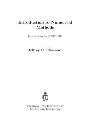
  • 45. 6.4. ADAPTIVE INTEGRATION 39 푎 푑 푐 푒 푏 Figure 6.1: Adaptive Simpson quadrature: Level 1. More important is the Global Error which is obtained from the composite formula (6.7) for the trapezoidal rule. Putting in the remainder terms, we have ∫︁ 푏 푎 푓(푥)푑푥 = ℎ 2 (푓0 + 2푓1 + · · · + 2푓푛−1 + 푓푛) − ℎ3 12 푛Σ︁−1 푖=0 푓′′(휉푖), where 휉푖 are values satisfying 푥푖 ≤ 휉푖 ≤ 푥푖+1. The remainder can be rewritten as − ℎ3 12 푛Σ︁−1 푖=0 푓′′(휉푖) = − 푛ℎ3 12 ⟨︀ 푓′′(휉푖) ⟩︀ , where ⟨︀ 푓′′(휉푖) ⟩︀ is the average value of all the 푓′′(휉푖)’s. Now, 푛 = 푏 − 푎 ℎ , so that the error term becomes − 푛ℎ3 12 ⟨︀ 푓′′(휉푖) ⟩︀ = − (푏 − 푎)ℎ2 12 ⟨︀ 푓′′(휉푖) ⟩︀ = O(ℎ2). Therefore, the global error is O(ℎ2). That is, a halving of the grid spacing only decreases the global error by a factor of four. Similarly, Simpson’s rule has a local error of O(ℎ5) and a global error of O(ℎ4). 6.4 Adaptive integration The useful MATLAB function quad.m performs numerical integration using adaptive Simpson quadrature. The idea is to let the computation itself decide on the grid size required to achieve a certain level of accuracy. Moreover, the grid size need not be the same over the entire region of integration. We begin the adaptive integration at what is called Level 1. The uniformly spaced points at which the function 푓(푥) is to be evaluated are shown in Fig. 6.1. The distance between the points 푎 and 푏 is taken to be 2ℎ, so that ℎ = 푏 − 푎 2 .
  • 46. 40 CHAPTER 6. INTEGRATION Integration using Simpson’s rule (6.5) with grid size ℎ yields 퐼 = ℎ 3 (︀ 푓(푎) + 4푓(푐) + 푓(푏) )︀ − ℎ5 90 푓′′′′(휉), where 휉 is some value satisfying 푎 ≤ 휉 ≤ 푏. Integration using Simpson’s rule twice with grid size ℎ/2 yields 퐼 = ℎ 6 (︀ 푓(푎) + 4푓(푑) + 2푓(푐) + 4푓(푒) + 푓(푏) )︀ − (ℎ/2)5 90 푓′′′′(휉푙) − (ℎ/2)5 90 푓′′′′(휉푟), with 휉푙 and 휉푟 some values satisfying 푎 ≤ 휉푙 ≤ 푐 and 푐 ≤ 휉푟 ≤ 푏. We now define 푆1 = ℎ 3 (︀ 푓(푎) + 4푓(푐) + 푓(푏) )︀ , 푆2 = ℎ 6 (︀ 푓(푎) + 4푓(푑) + 2푓(푐) + 4푓(푒) + 푓(푏) )︀ , 퐸1 = − ℎ5 90 푓′′′′(휉), 퐸2 = − ℎ5 25 · 90 (︀ 푓′′′′(휉푙) + 푓′′′′(휉푟) )︀ . Now we ask whether 푆2 is accurate enough, or must we further refine the cal-culation and go to Level 2? To answer this question, we make the simplifying approximation that all of the fourth-order derivatives of 푓(푥) in the error terms are equal; that is, 푓′′′′(휉) = 푓′′′′(휉푙) = 푓′′′′(휉푟) = 퐶. Then 퐸1 = − ℎ5 90 퐶, 퐸2 = − ℎ5 24 · 90 퐶 = 1 16 퐸1. Then since 푆1 + 퐸1 = 푆2 + 퐸2, and 퐸1 = 16퐸2, we have for our estimate for the error term 퐸2, 퐸2 = 1 15 (푆2 − 푆1). Therefore, given some specific value of the tolerance tol, if ⃒⃒⃒⃒ 1 15 ⃒⃒⃒⃒ (푆2 − 푆1) tol, then we can accept 푆2 as 퐼. If the tolerance is not achieved for 퐼, then we proceed to Level 2. The computation at Level 2 further divides the integration interval from 푎 to 푏 into the two integration intervals 푎 to 푐 and 푐 to 푏, and proceeds with the
  • 47. 6.4. ADAPTIVE INTEGRATION 41 above procedure independently on both halves. Integration can be stopped on either half provided the tolerance is less than tol/2 (since the sum of both errors must be less than tol). Otherwise, either half can proceed to Level 3, and so on. As a side note, the two values of 퐼 given above (for integration with step size ℎ and ℎ/2) can be combined to give a more accurate value for I given by 퐼 = 16푆2 − 푆1 15 + O(ℎ7), where the error terms of O(ℎ5) approximately cancel. This free lunch, so to speak, is called Richardson’s extrapolation.
  • 48. 42 CHAPTER 6. INTEGRATION
  • 49. Chapter 7 Ordinary differential equations We now discuss the numerical solution of ordinary differential equations. These include the initial value problem, the boundary value problem, and the eigen-value problem. Before proceeding to the development of numerical methods, we review the analytical solution of some classic equations. 7.1 Examples of analytical solutions 7.1.1 Initial value problem One classic initial value problem is the 푅퐶 circuit. With 푅 the resistor and 퐶 the capacitor, the differential equation for the charge 푞 on the capacitor is given by 푅 푑푞 푑푡 + 푞 퐶 = 0. (7.1) If we consider the physical problem of a charged capacitor connected in a closed circuit to a resistor, then the initial condition is 푞(0) = 푞0, where 푞0 is the initial charge on the capacitor. The differential equation (7.1) is separable, and separating and integrating from time 푡 = 0 to 푡 yields ∫︁ 푞 푞0 푑푞 푞 = − 1 푅퐶 ∫︁ 푡 0 푑푡, which can be integrated and solved for 푞 = 푞(푡): 푞(푡) = 푞0푒−푡/푅퐶. The classic second-order initial value problem is the 푅퐿퐶 circuit, with dif-ferential equation 퐿 푑2푞 푑푡2 + 푅 푑푞 푑푡 + 푞 퐶 = 0. Here, a charged capacitor is connected to a closed circuit, and the initial condi-tions satisfy 푞(0) = 푞0, 푑푞 푑푡 (0) = 0. 43
  • 50. 44 CHAPTER 7. ORDINARY DIFFERENTIAL EQUATIONS The solution is obtained for the second-order equation by the ansatz 푞(푡) = 푒푟푡, which results in the following so-called characteristic equation for 푟: 퐿푟2 + 푅푟 + 1 퐶 = 0. If the two solutions for 푟 are distinct and real, then the two found exponential solutions can be multiplied by constants and added to form a general solution. The constants can then be determined by requiring the general solution to satisfy the two initial conditions. If the roots of the characteristic equation are complex or degenerate, a general solution to the differential equation can also be found. 7.1.2 Boundary value problems The dimensionless equation for the temperature 푦 = 푦(푥) along a linear heat-conducting rod of length unity, and with an applied external heat source 푓(푥), is given by the differential equation − 푑2푦 푑푥2 = 푓(푥), (7.2) with 0 ≤ 푥 ≤ 1. Boundary conditions are usually prescribed at the end points of the rod, and here we assume that the temperature at both ends are maintained at zero so that 푦(0) = 0, 푦(1) = 0. The assignment of boundary conditions at two separate points is called a two-point boundary value problem, in contrast to the initial value problem where the boundary conditions are prescribed at only a single point. Two-point boundary value problems typically require a more sophisticated algorithm for a numerical solution than initial value problems. Here, the solution of (7.2) can proceed by integration once 푓(푥) is specified. We assume that 푓(푥) = 푥(1 − 푥), so that the maximum of the heat source occurs in the center of the rod, and goes to zero at the ends. The differential equation can then be written as 푑2푦 푑푥2 = −푥(1 − 푥). The first integration results in 푑푦 푑푥 = ∫︁ (푥2 − 푥)푑푥 = 푥3 3 − 푥2 2 + 푐1,
  • 51. 7.1. EXAMPLES OF ANALYTICAL SOLUTIONS 45 where 푐1 is the first integration constant. Integrating again, 푦(푥) = ∫︁ (︂ 푥3 3 − 푥2 2 + 푐1 )︂ 푑푥 = 푥4 12 − 푥3 6 + 푐1푥 + 푐2, where 푐2 is the second integration constant. The two integration constants are determined by the boundary conditions. At 푥 = 0, we have 0 = 푐2, and at 푥 = 1, we have 0 = 1 12 − 1 6 + 푐1, so that 푐1 = 1/12. Our solution is therefore 푦(푥) = 푥4 12 − 푥3 6 + 푥 12 = 1 12 푥(1 − 푥)(1 + 푥 − 푥2). The temperature of the rod is maximum at 푥 = 1/2 and goes smoothly to zero at the ends. 7.1.3 Eigenvalue problem The classic eigenvalue problem obtained by solving the wave equation by sepa-ration of variables is given by 푑2푦 푑푥2 + 휆2푦 = 0, with the two-point boundary conditions 푦(0) = 0 and 푦(1) = 0. Notice that 푦(푥) = 0 satisfies both the differential equation and the boundary conditions. Other nonzero solutions for 푦 = 푦(푥) are possible only for certain discrete values of 휆. These values of 휆 are called the eigenvalues of the differential equation. We proceed by first finding the general solution to the differential equation. It is easy to see that this solution is 푦(푥) = 퐴cos 휆푥 + 퐵 sin 휆푥. Imposing the first boundary condition at 푥 = 0, we obtain 퐴 = 0. The second boundary condition at 푥 = 1 results in 퐵 sin 휆 = 0. Since we are searching for a solution where 푦 = 푦(푥) is not identically zero, we must have 휆 = 휋, 2휋, 3휋, . . . .
  • 52. 46 CHAPTER 7. ORDINARY DIFFERENTIAL EQUATIONS The corresponding negative values of 휆 are also solutions, but their inclusion only changes the corresponding values of the unknown 퐵 constant. A linear superposition of all the solutions results in the general solution 푦(푥) = ∞Σ︁ 푛=1 퐵푛 sin 푛휋푥. For each eigenvalue 푛휋, we say there is a corresponding eigenfunction sin 푛휋푥. When the differential equation can not be solved analytically, a numerical method should be able to solve for both the eigenvalues and eigenfunctions. 7.2 Numerical methods: initial value problem We begin with the simple Euler method, then discuss the more sophisticated Runge-Kutta methods, and conclude with the Runge-Kutta-Fehlberg method, as implemented in the MATLAB function ode45.m. Our differential equations are for 푥 = 푥(푡), where the time 푡 is the independent variable, and we will make use of the notation 푥˙ = 푑푥/푑푡. This notation is still widely used by physicists and descends directly from the notation originally used by Newton. 7.2.1 Euler method The Euler method is the most straightforward method to integrate a differential equation. Consider the first-order differential equation 푥˙ = 푓(푡, 푥), (7.3) with the initial condition 푥(0) = 푥0. Define 푡푛 = 푛Δ푡 and 푥푛 = 푥(푡푛). A Taylor series expansion of 푥푛+1 results in 푥푛+1 = 푥(푡푛 + Δ푡) = 푥(푡푛) + Δ푡푥˙ (푡푛) + O(Δ푡2) = 푥(푡푛) + Δ푡푓 (푡푛, 푥푛) + O(Δ푡2). The Euler Method is therefore written as 푥푛+1 = 푥(푡푛) + Δ푡푓 (푡푛, 푥푛). We say that the Euler method steps forward in time using a time-step Δ푡, starting from the initial value 푥0 = 푥(0). The local error of the Euler Method is O(Δ푡2). The global error, however, incurred when integrating to a time 푇, is a factor of 1/Δ푡 larger and is given by O(Δ푡). It is therefore customary to call the Euler Method a first-order method. 7.2.2 Modified Euler method This method is of a type that is called a predictor-corrector method. It is also the first of what are Runge-Kutta methods. As before, we want to solve (7.3). The idea is to average the value of 푥˙ at the beginning and end of the time step. That is, we would like to modify the Euler method and write 푥푛+1 = 푥푛 + 1 2 Δ푡 (︀ 푓(푡푛, 푥푛) + 푓(푡푛 + Δ푡, 푥푛+1) )︀ .
  • 53. 7.2. NUMERICAL METHODS: INITIAL VALUE PROBLEM 47 The obvious problem with this formula is that the unknown value 푥푛+1 appears on the right-hand-side. We can, however, estimate this value, in what is called the predictor step. For the predictor step, we use the Euler method to find 푥푝 푛+1 = 푥푛 + Δ푡푓 (푡푛, 푥푛). The corrector step then becomes 푥푛+1 = 푥푛 + 1 2 Δ푡 (︀ 푓(푡푛, 푥푛) + 푓(푡푛 + Δ푡, 푥푝 푛+1) )︀ . The Modified Euler Method can be rewritten in the following form that we will later identify as a Runge-Kutta method: 푘1 = Δ푡푓 (푡푛, 푥푛), 푘2 = Δ푡푓 (푡푛 + Δ푡, 푥푛 + 푘1), 푥푛+1 = 푥푛 + 1 2 (푘1 + 푘2). (7.4) 7.2.3 Second-order Runge-Kutta methods We now derive all second-order Runge-Kutta methods. Higher-order methods can be similarly derived, but require substantially more algebra. We consider the differential equation given by (7.3). A general second-order Runge-Kutta method may be written in the form 푘1 = Δ푡푓 (푡푛, 푥푛), 푘2 = Δ푡푓 (푡푛 + 훼Δ푡, 푥푛 + 훽푘1), 푥푛+1 = 푥푛 + 푎푘1 + 푏푘2, (7.5) with 훼, 훽, 푎 and 푏 constants that define the particular second-order Runge- Kutta method. These constants are to be constrained by setting the local error of the second-order Runge-Kutta method to be O(Δ푡3). Intuitively, we might guess that two of the constraints will be 푎 + 푏 = 1 and 훼 = 훽. We compute the Taylor series of 푥푛+1 directly, and from the Runge-Kutta method, and require them to be the same to order Δ푡2. First, we compute the Taylor series of 푥푛+1. We have 푥푛+1 = 푥(푡푛 + Δ푡) = 푥(푡푛) + Δ푡푥˙ (푡푛) + 1 2 (Δ푡)2¨푥(푡푛) + O(Δ푡3). Now, 푥˙ (푡푛) = 푓(푡푛, 푥푛). The second derivative is more complicated and requires partial derivatives. We have ¨푥(푡푛) = 푑 푑푡 푓(푡, 푥(푡)) ]︂ 푡=푡푛 = 푓푡(푡푛, 푥푛) + 푥˙ (푡푛)푓푥(푡푛, 푥푛) = 푓푡(푡푛, 푥푛) + 푓(푡푛, 푥푛)푓푥(푡푛, 푥푛).
  • 54. 48 CHAPTER 7. ORDINARY DIFFERENTIAL EQUATIONS Therefore, 푥푛+1 = 푥푛 + Δ푡푓 (푡푛, 푥푛) + 1 2 (Δ푡)2 (︀ 푓푡(푡푛, 푥푛) + 푓(푡푛, 푥푛)푓푥(푡푛, 푥푛) )︀ . (7.6) Second, we compute 푥푛+1 from the Runge-Kutta method given by (7.5). Substituting in 푘1 and 푘2, we have 푥푛+1 = 푥푛 + 푎Δ푡푓 (푡푛, 푥푛) + 푏Δ푡푓 (︀ 푡푛 + 훼Δ푡, 푥푛 + 훽Δ푡푓 (푡푛, 푥푛) )︀ . We Taylor series expand using 푓 (︀ 푡푛 + 훼Δ푡, 푥푛 + 훽Δ푡푓 (푡푛, 푥푛) )︀ = 푓(푡푛, 푥푛) + 훼Δ푡푓푡(푡푛, 푥푛) + 훽Δ푡푓 (푡푛, 푥푛)푓푥(푡푛, 푥푛) + O(Δ푡2). The Runge-Kutta formula is therefore 푥푛+1 = 푥푛 + (푎 + 푏)Δ푡푓 (푡푛, 푥푛) + (Δ푡)2(︀ 훼푏푓푡(푡푛, 푥푛) + 훽푏푓(푡푛, 푥푛)푓푥(푡푛, 푥푛) )︀ + O(Δ푡3). (7.7) Comparing (7.6) and (7.7), we find 푎 + 푏 = 1, 훼푏 = 1/2, 훽푏 = 1/2. There are three equations for four parameters, and there exists a family of second-order Runge-Kutta methods. The Modified Euler Method given by (7.4) corresponds to 훼 = 훽 = 1 and 푎 = 푏 = 1/2. Another second-order Runge-Kutta method, called the Midpoint Method, corresponds to 훼 = 훽 = 1/2, 푎 = 0 and 푏 = 1. This method is written as 푘1 = Δ푡푓 (푡푛, 푥푛), 푘2 = Δ푡푓 (︂ 푡푛 + 1 2 Δ푡, 푥푛 + 1 2 푘1 )︂ , 푥푛+1 = 푥푛 + 푘2. 7.2.4 Higher-order Runge-Kutta methods The general second-order Runge-Kutta method was given by (7.5). The general form of the third-order method is given by 푘1 = Δ푡푓 (푡푛, 푥푛), 푘2 = Δ푡푓 (푡푛 + 훼Δ푡, 푥푛 + 훽푘1), 푘3 = Δ푡푓 (푡푛 + 훾Δ푡, 푥푛 + 훿푘1 + 휖푘2), 푥푛+1 = 푥푛 + 푎푘1 + 푏푘2 + 푐푘3. The following constraints on the constants can be guessed: 훼 = 훽, 훾 = 훿 + 휖, and 푎 + 푏 + 푐 = 1. Remaining constraints need to be derived.
  • 55. 7.2. NUMERICAL METHODS: INITIAL VALUE PROBLEM 49 The fourth-order method has a 푘1, 푘2, 푘3 and 푘4. The fifth-order method requires up to 푘6. The table below gives the order of the method and the number of stages required. order 2 3 4 5 6 7 8 minimum # stages 2 3 4 6 7 9 11 Because of the jump in the number of stages required between the fourth-order and fifth-order method, the fourth-order Runge-Kutta method has some appeal. The general fourth-order method starts with 13 constants, and one then finds 11 constraints. A particularly simple fourth-order method that has been widely used is given by 푘1 = Δ푡푓 (푡푛, 푥푛), 푘2 = Δ푡푓 (︂ 푡푛 + 1 2 Δ푡, 푥푛 + 1 2 푘1 )︂ , 푘3 = Δ푡푓 (︂ 푡푛 + 1 2 Δ푡, 푥푛 + 1 2 푘2 )︂ , 푘4 = Δ푡푓 (푡푛 + Δ푡, 푥푛 + 푘3) , 푥푛+1 = 푥푛 + 1 6 (푘1 + 2푘2 + 2푘3 + 푘4) . 7.2.5 Adaptive Runge-Kutta Methods As in adaptive integration, it is useful to devise an ode integrator that au-tomatically finds the appropriate Δ푡. The Dormand-Prince Method, which is implemented in MATLAB’s ode45.m, finds the appropriate step size by compar-ing the results of a fifth-order and fourth-order method. It requires six function evaluations per time step, and constructs both a fifth-order and a fourth-order method from these function evaluations. Suppose the fifth-order method finds 푥푛+1 with local error O(Δ푡6), and the fourth-order method finds 푥′ 푛+1 with local error O(Δ푡5). Let 휀 be the desired error tolerance of the method, and let 푒 be the actual error. We can estimate 푒 from the difference between the fifth- and fourth-order methods; that is, 푒 = |푥푛+1 − 푥′ 푛+1|. Now 푒 is of O(Δ푡5), where Δ푡 is the step size taken. Let Δ휏 be the estimated step size required to get the desired error 휀. Then we have 푒/휀 = (Δ푡)5/(Δ휏 )5, or solving for Δ휏 , Δ휏 = Δ푡 (︁휀 푒 )︁1/5 . On the one hand, if 푒 휀, then we accept 푥푛+1 and do the next time step using the larger value of Δ휏 . On the other hand, if 푒 휀, then we reject the integration step and redo the time step using the smaller value of Δ휏 . In practice, one usually increases the time step slightly less and decreases the time step slightly more to prevent the waste of too many failed time steps.
  • 56. 50 CHAPTER 7. ORDINARY DIFFERENTIAL EQUATIONS 7.2.6 System of differential equations Our numerical methods can be easily adapted to solve higher-order differential equations, or equivalently, a system of differential equations. First, we show how a second-order differential equation can be reduced to two first-order equations. Consider 푥¨ = 푓(푡, 푥, 푥˙ ). This second-order equation can be rewritten as two first-order equations by defining 푢 = 푥˙ . We then have the system 푥˙ = 푢, 푢˙ = 푓(푡, 푥, 푢). This trick also works for higher-order equation. For another example, the third-order equation ... 푥 = 푓(푡, 푥, 푥˙ , 푥¨), can be written as 푥˙ = 푢, 푢˙ = 푣, 푣˙ = 푓(푡, 푥, 푢, 푣). Now, we show how to generalize Runge-Kutta methods to a system of dif-ferential equations. As an example, consider the following system of two odes, 푥˙ = 푓(푡, 푥, 푦), 푦˙ = 푔(푡, 푥, 푦), with the initial conditions 푥(0) = 푥0 and 푦(0) = 푦0. The generalization of the
  • 57. 7.3. NUMERICAL METHODS: BOUNDARY VALUE PROBLEM 51 commonly used fourth-order Runge-Kutta method would be 푘1 = Δ푡푓 (푡푛, 푥푛, 푦푛), 푙1 = Δ푡푔(푡푛, 푥푛, 푦푛), 푘2 = Δ푡푓 (︂ 푡푛 + 1 2 Δ푡, 푥푛 + 1 2 푘1, 푦푛 + 1 2 푙1 )︂ , 푙2 = Δ푡푔 (︂ 푡푛 + 1 2 Δ푡, 푥푛 + 1 2 푘1, 푦푛 + 1 2 푙1 )︂ , 푘3 = Δ푡푓 (︂ 푡푛 + 1 2 Δ푡, 푥푛 + 1 2 푘2, 푦푛 + 1 2 푙2 )︂ , 푙3 = Δ푡푔 (︂ 푡푛 + 1 2 Δ푡, 푥푛 + 1 2 푘2, 푦푛 + 1 2 푙2 )︂ , 푘4 = Δ푡푓 (푡푛 + Δ푡, 푥푛 + 푘3, 푦푛 + 푙3) , 푙4 = Δ푡푔 (푡푛 + Δ푡, 푥푛 + 푘3, 푦푛 + 푙3) , 푥푛+1 = 푥푛 + 1 6 (푘1 + 2푘2 + 2푘3 + 푘4) , 푦푛+1 = 푦푛 + 1 6 (푙1 + 2푙2 + 2푙3 + 푙4) . 7.3 Numerical methods: boundary value prob-lem 7.3.1 Finite difference method We consider first the differential equation − 푑2푦 푑푥2 = 푓(푥), 0 ≤ 푥 ≤ 1, (7.8) with two-point boundary conditions 푦(0) = 퐴, 푦(1) = 퐵. Equation (7.8) can be solved by quadrature, but here we will demonstrate a numerical solution using a finite difference method. We begin by discussing how to numerically approximate derivatives. Con-sider the Taylor series approximation for 푦(푥 + ℎ) and 푦(푥 − ℎ), given by 푦(푥 + ℎ) = 푦(푥) + ℎ푦′(푥) + 1 2 ℎ2푦′′(푥) + 1 6 ℎ3푦′′′(푥) + 1 24 ℎ4푦′′′′(푥) + . . . , 푦(푥 − ℎ) = 푦(푥) − ℎ푦′(푥) + 1 2 ℎ2푦′′(푥) − 1 6 ℎ3푦′′′(푥) + 1 24 ℎ4푦′′′′(푥) + . . . .
  • 58. 52 CHAPTER 7. ORDINARY DIFFERENTIAL EQUATIONS The standard definitions of the derivatives give the first-order approximations 푦′(푥) = 푦(푥 + ℎ) − 푦(푥) ℎ + O(ℎ), 푦′(푥) = 푦(푥) − 푦(푥 − ℎ) ℎ + O(ℎ). The more widely-used second-order approximation is called the central differ-ence approximation and is given by 푦′(푥) = 푦(푥 + ℎ) − 푦(푥 − ℎ) 2ℎ + O(ℎ2). The finite difference approximation to the second derivative can be found from considering 푦(푥 + ℎ) + 푦(푥 − ℎ) = 2푦(푥) + ℎ2푦′′(푥) + 1 12 ℎ4푦′′′′(푥) + . . . , from which we find 푦′′(푥) = 푦(푥 + ℎ) − 2푦(푥) + 푦(푥 − ℎ) ℎ2 + O(ℎ2). Sometimes a second-order method is required for 푥 on the boundaries of the domain. For a boundary point on the left, a second-order forward difference method requires the additional Taylor series 푦(푥 + 2ℎ) = 푦(푥) + 2ℎ푦′(푥) + 2ℎ2푦′′(푥) + 4 3 ℎ3푦′′′(푥) + . . . . We combine the Taylor series for 푦(푥 + ℎ) and 푦(푥 + 2ℎ) to eliminate the term proportional to ℎ2: 푦(푥 + 2ℎ) − 4푦(푥 + ℎ) = −3푦(푥) − 2ℎ푦′(푥) + O(h3). Therefore, 푦′(푥) = −3푦(푥) + 4푦(푥 + ℎ) − 푦(푥 + 2ℎ) 2ℎ + O(ℎ2). For a boundary point on the right, we send ℎ → −ℎ to find 푦′(푥) = 3푦(푥) − 4푦(푥 − ℎ) + 푦(푥 − 2ℎ) 2ℎ + O(ℎ2). We now write a finite difference scheme to solve (7.8). We discretize 푥 by defining 푥푖 = 푖ℎ, 푖 = 0, 1, . . . , 푛 + 1. Since 푥푛+1 = 1, we have ℎ = 1/(푛 + 1). The functions 푦(푥) and 푓(푥) are discretized as 푦푖 = 푦(푥푖) and 푓푖 = 푓(푥푖). The second-order differential equation (7.8) then becomes for the interior points of the domain −푦푖−1 + 2푦푖 − 푦푖+1 = ℎ2푓푖, 푖 = 1, 2, . . . 푛, with the boundary conditions 푦0 = 퐴 and 푦푛+1 = 퐵. We therefore have a linear system of equations to solve. The first and 푛th equation contain the boundary conditions and are given by 2푦1 − 푦2 = ℎ2푓1 + 퐴, −푦푛−1 + 2푦푛 = ℎ2푓푛 + 퐵.
  • 59. 7.3. NUMERICAL METHODS: BOUNDARY VALUE PROBLEM 53 The second and third equations, etc., are −푦1 + 2푦2 − 푦3 = ℎ2푓2, −푦2 + 2푦3 − 푦4 = ℎ2푓3, . . . In matrix form, we have ⎛ ⎜⎜⎜⎜⎜⎜⎜⎝ ⎞ 2 −1 0 0 . . . 0 0 0 −1 2 −1 0 . . . 0 0 0 0 −1 2 −1 . . . 0 0 0 ... ... ... ... . . . ... ... ... ⎟⎟⎟⎟⎟⎟⎟⎠ 0 0 0 0 . . . −1 2 −1 0 0 0 0 . . . 0 −1 2 ⎛ ⎜⎜⎜⎜⎜⎜⎜⎝ 푦1 푦2 푦3 ... 푦푛−1 푦푛 ⎞ ⎟⎟⎟⎟⎟⎟⎟⎠ = ⎛ ⎜⎜⎜⎜⎜⎜⎜⎝ ℎ2푓1 + 퐴 ℎ2푓2 ℎ2푓3 ... ℎ2푓푛−1 ℎ2푓푛 + 퐵 ⎞ ⎟⎟⎟⎟⎟⎟⎟⎠ . The matrix is tridiagonal, and a numerical solution by Guassian elimination can be done quickly. The matrix itself is easily constructed using the MATLAB function diag.m and ones.m. As excerpted from the MATLAB help page, the function call ones(m,n) returns an m-by-n matrix of ones, and the function call diag(v,k), when v is a vector with n components, is a square matrix of order n+abs(k) with the elements of v on the k-th diagonal: 푘 = 0 is the main diag-onal, 푘 0 is above the main diagonal and 푘 0 is below the main diagonal. The 푛 × 푛 matrix above can be constructed by the MATLAB code M=diag(-ones(n-1,1),-1)+diag(2*ones(n,1),0)+diag(-ones(n-1,1),1); . The right-hand-side, provided f is a given n-by-1 vector, can be constructed by the MATLAB code b=h^2*f; b(1)=b(1)+A; b(n)=b(n)+B; and the solution for u is given by the MATLAB code y=M∖b; 7.3.2 Shooting method The finite difference method can solve linear odes. For a general ode of the form 푑2푦 푑푥2 = 푓(푥, 푦, 푑푦/푑푥), with 푦(0) = 퐴 and 푦(1) = 퐵, we use a shooting method. First, we formulate the ode as an initial value problem. We have 푑푦 푑푥 = 푧, 푑푧 푑푥 = 푓(푥, 푦, 푧).
  • 60. 54 CHAPTER 7. ORDINARY DIFFERENTIAL EQUATIONS The initial condition 푦(0) = 퐴 is known, but the second initial condition 푧(0) = 푏 is unknown. Our goal is to determine 푏 such that 푦(1) = 퐵. In fact, this is a root-finding problem for an appropriately defined function. We define the function 퐹 = 퐹(푏) such that 퐹(푏) = 푦(1) − 퐵. In other words, 퐹(푏) is the difference between the value of 푦(1) obtained from integrating the differential equations using the initial condition 푧(0) = 푏, and 퐵. Our root-finding routine will want to solve 퐹(푏) = 0. (The method is called shooting because the slope of the solution curve for 푦 = 푦(푥) at 푥 = 0 is given by 푏, and the solution hits the value 푦(1) at 푥 = 1. This looks like pointing a gun and trying to shoot the target, which is 퐵.) To determine the value of 푏 that solves 퐹(푏) = 0, we iterate using the Secant method, given by 푏푛+1 = 푏푛 − 퐹(푏푛) 푏푛 − 푏푛−1 퐹(푏푛) − 퐹(푏푛−1) . We need to start with two initial guesses for 푏, solving the ode for the two corresponding values of 푦(1). Then the Secant Method will give us the next value of 푏 to try, and we iterate until |푦(1) − 퐵| tol, where tol is some specified tolerance for the error. 7.4 Numerical methods: eigenvalue problem For illustrative purposes, we develop our numerical methods for what is perhaps the simplest eigenvalue ode. With 푦 = 푦(푥) and 0 ≤ 푥 ≤ 1, this simple ode is given by 푦′′ + 휆2푦 = 0. (7.9) To solve (7.9) numerically, we will develop both a finite difference method and a shooting method. Furthermore, we will show how to solve (7.9) with homo-geneous boundary conditions on either the function 푦 or its derivative 푦′. 7.4.1 Finite difference method We first consider solving (7.9) with the homogeneous boundary conditions 푦(0) = 푦(1) = 0. In this case, we have already shown that the eigenvalues of (7.9) are given by 휆 = 휋, 2휋, 3휋, . . . . With 푛 interior points, we have 푥푖 = 푖ℎ for 푖 = 0, . . . , 푛 + 1, and ℎ = 1/(푛 + 1). Using the centered-finite-difference approximation for the second derivative, (7.9) becomes 푦푖−1 − 2푦푖 + 푦푖+1 = −ℎ2휆2푦푖. (7.10) Applying the boundary conditions 푦0 = 푦푛+1 = 0, the first equation with 푖 = 1, and the last equation with 푖 = 푛, are given by −2푦1 + 푦2 = −ℎ2휆2푦1, 푦푛−1 − 2푦푛 = −ℎ2휆2푦푛.
  • 61. 7.4. NUMERICAL METHODS: EIGENVALUE PROBLEM 55 The remaining 푛 − 2 equations are given by (7.10) for 푖 = 2, . . . , 푛 − 1. It is of interest to see how the solution develops with increasing 푛. The smallest possible value is 푛 = 1, corresponding to a single interior point, and since ℎ = 1/2 we have −2푦1 = − 1 4 휆2푦1, so that 휆2 = 8, or 휆 = 2 √ 2 = 2.8284. This is to be compared to the first eigenvalue which is 휆 = 휋. When 푛 = 2, we have ℎ = 1/3, and the resulting two equations written in matrix form are given by (︂ −2 1 )︂(︂ 1 −2 푦1 푦2 )︂ = − 1 9 휆2 (︂ 푦1 푦2 )︂ . This is a matrix eigenvalue problem with the eigenvalue given by 휇 = −휆2/9. The solution for 휇 is arrived at by solving det (︂ −2 − 휇 1 )︂ 1 −2 − 휇 = 0, with resulting quadratic equation (2 + 휇)2 − 1 = 0. √ −휇, we have 휆 = 3, 3 The solutions are 휇 = −1,−3, and since 휆 = 3 √ 3 = 5.1962. These two eigenvalues serve as rough approximations to the first two eigenvalues 휋 and 2휋. With A an 푛-by-푛 matrix, the MATLAB variable mu=eig(A) is a vector containing the 푛 eigenvalues of the matrix A. The built-in function eig.m can therefore be used to find the eigenvalues. With 푛 grid points, the smaller eigen-values will converge more rapidly than the larger ones. We can also consider boundary conditions on the derivative, or mixed bound-ary conditions. For example, consider the mixed boundary conditions given by 푦(0) = 0 and 푦′(1) = 0. The eigenvalues of (7.9) can then be determined analytically to be 휆푖 = (푖 − 1/2)휋, with 푖 a natural number. The difficulty we now face is how to implement a boundary condition on the derivative. Our computation of 푦′′ uses a second-order method, and we would like the computation of the first derivative to also be second order. The condition 푦′(1) = 0 occurs on the right-most boundary, and we can make use of the second-order backward-difference approximation to the derivative that we have previously derived. This finite-difference approximation for 푦′(1) can be written as 푦′ 푛+1 = 3푦푛+1 − 4푦푛 + 푦푛−1 2ℎ . (7.11) Now, the 푛th finite-difference equation was given by 푦푛−1 − 2푦푛 + 푦푛+1 = −ℎ2푦푛, and we now replace the value 푦푛+1 using (7.11); that is, 푦푛+1 = 1 3 (︀ 2ℎ푦′푛 +1 + 4푦푛 − 푦푛−1 )︀ .