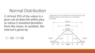
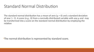
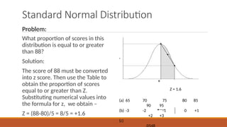
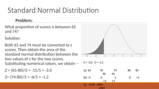
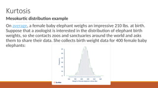
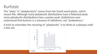
Normal distribution.pptx aaaaaaaaaaaaaaa

CONCEPT OF NORMAL DISTRIBUTION
 A theoretical concept whose objective is to be able to explain
for some variables the relation between the intervals of its
values and their corresponding probabilities.
 The graph of a normally distributed set of data is bell-shaped
and is symmetric around a vertical line created at the center.
 The curve has two tails on both sides that extend indefinitely in
opposite direction.
 The two tails do not intersect with the horizontal axis.

Normal Distribution
The curve of a normally
distributed set of data can be
described by the value of the
mean and the standard
deviation.
We shall consider three specific
intervals with which we can
associate three mathematical
facts called the Empirical Rule.
GRAPH OF A NORMALLY DISTRIBUTED SET OF
DATA

Normal Distribution
1. At least 68% of the values in
the given set of data fall within
plus or minus 1 standard
deviation from the mean. In
symbols, the interval is given by
◦( – 1s) – ( + 1s)
SUBDIVISION OF THE HORIZONTAL AXIS INTO EQUAL SUB-
INTERVALS WITH 1 UNIT EQUAL TO 1 STANDARD
DEVIATION

Normal Distribution
2. At least 95% of the values in a
given set of data fall within plus
or minus 2 standard deviation
from the mean. In symbols, the
interval is given by
◦( – 2s) – ( + 2s)
DEVIATION

Normal Distribution
3. At least 99% of the values in a
given set of data fall within plus
or minus 3 standard deviation
from the mean. In symbols, the
interval is given by
◦( – 3s) – ( + 3s)
DEVIATION

Significance of the Empirical Rule
Consider the NCEE scores of the
students in a certain college whose
mean score is 75 and a standard
deviation of 8. Assuming normality of
the data, we can say that
a) Approximately, 68% of the students
in that college have NCEE scores
between 75 plus or minus 8, that is,
◦(– 1(8) – (+ 1(8)
◦ 67 – 83
THE APPROXIMATE AREAS OF THE INTERVALS
REPRESENTING THE EMPIRICAL RULE

b) Approximately, 95% of the
students in that college have
NCEE scores between 75 plus
or minus 2 times the standard
deviation, 8. Thus,
◦(– 2(8) – (+ 2(8)
◦ 75 – 16 – 75 + 16
◦ 59 – 91
THE APPROXIMATE AREAS OF THE INTERVALS
REPRESENTING THE EMPIRICAL RULE

c) Approximately, 99% of the
students in that college have
NCEE scores between 75 plus
or minus 3 times the standard
deviation, 8. Thus,
◦(– 3(8) – (+ 3(8)
◦ 75 – 24 – 75 + 24
◦ 51 – 99
THE GRAPH OF THE NCEE SCORES OF THE
STUDENTS IN A CERTAIN COLLEGE
51 59 67 75 83
91 99

Properties of the Normal Distribution
1. Symmetrical. A theoretical normal distribution is symmetrical about its mode,
median, and mean. In a normal distribution, then, the mode, median, and mean are
equal to each other.
2. Asymptotic. The tails of the normal distribution approach closer to the base line, or
abscissa, as they get farther away from µ. The distribution, however, is asymptotic;
the tails never touch the base line, regardless of the distance from µ.
3. Continuous. The normal distribution is continuous for all scores between plus and
minus infinity. This means that, for any two scores, I can always obtain another
score that lies between them.

Area under the Normal Distribution
 In normal distribution, specific
proportions of scores are within
certain intervals about the mean.
 In any normally distributed
population, .3413 of the scores is in
an internal between µ and µ plus one
standard deviation.
 The proportion .3413 can be
expressed as a percent by multiplying
it by 100; thus .3413 equals 34.13
percent.
Subdivision of the horizontal axis into equal sub-
intervals with 1 unit equal to 1 standard deviation

Area under the Normal Distribution
To summarize, in a normal distribution the following relations hold between
µ, , the proportion of scores, and the percentage of scores contained in
certain intervals about the mean:
Interval Proportion of Scores in Interval Percentage of Scores in Interval
µ - 1 to µ + 1 .6826 68.26
µ - 2 to µ + 2 .9544 95.44
µ - 3 to µ + 3 .9974 99.74

Standard Normal Distribution
The standard normal distribution has a mean of zero (µ = 0) and a standard deviation
of one ( = 1). A score (e.g., X) from a normally distributed variable with any µ and may
be transformed into a score on the standard normal distribution by employing the
relation
◦The normal distribution is represented by standard score.

Standard Score
A standard score indicates how many standard deviations a
datum is above or below the population/sample mean.
It is derived by subtracting the population/sample mean
from an individual raw score and then dividing the difference
by the population/sample standard deviation (Moore, 2009).
The standard score is:
where:
x is a raw score to be standardized.
μ is the population mean.
σ is the population standard deviation.

Standard Normal Distribution (SND)
To demonstrate SND, suppose that a
score of 115 (i.e., X = 115) is obtained
from a normally distributed set of
scores with µ = 100 and =15. This
score is converted to a z score by
= +1.0

Location of a score of 115 from a
normal distribution with µ = 100
and = 15 on the standard normal
distribution. The labels on the X
axis show (a) the raw scores, (b) z
scores corresponding to the raw
scores, and (c) the proportion of
scores from z = -∞ to z = 0 and
from z = 0 to z = +1.
(a) 55 70 85 100 115
130 145
(b) -3 -2 -1 0 +1
+2 +3
(c) .5000
Z = + 1.0

What proportion of scores in this
distribution is equal to or less
than 82? Again convert 82 to a z
score, Z = (82 – 100)/15 = - 1.2.
This z score indicates that a score
of82 is 1.2 standard deviations
below the mean of the
distribution. The raw scores of
the distribution and the z = -1.2
as shown in the Figure. (a) 55 70 85 100 115
130 145
(b) -3 -2 -1 0 +1
+2 +3
(c) .1151
Z = - 1.2
Problem:

distribution is equal to or greater
than 88?
Solution:
The score of 88 must be converted
into z score. Then use the Table to
obtain the proportion of scores
equal to or greater than Z.
Substituting numerical values into
the formula for z, we obtain –
Z = (88-80)/5 = 8/5 = +1.6
(a) 65 70 75 80 85
90 95
(b) -3 -2 -1 0 +1
+2 +3
(c)
Z = 1.6
Problem:

distribution is between 83 and 87?
Solution:
Both 83 and 87 must be converted to z
scores. Then obtain the area of the
standard normal distribution between
the two values of z. Substituting
numerical values, we obtain –
Z = (83-80)/5 = 3/5 = +0.6
Z= (87-80)/5 = 7/5 = +1.4
(a) 65 70 75 80 85
90 95
(b) -3 -2 -1 0 +1
+2 +3
(c)
Z = 0.6 Z = +1.4
Problem:

What proportion of scores is between 65
and 74?
Solution:
Both 65 and 74 must be converted to z
scores. Then obtain the area of the
standard normal distribution between the
two values of z for the two scores.
Substituting numerical values, we obtain –
Z = (65-80)/5 = -15/5 = -3.0
Z= (74-80)/5 = -6/5 = -1.2
(a) 65 70 75 80 85
90 95
(b) -3 -2 -1 0 +1
+2 +3
(c) .1138 .3849
Z = -3.0 Z = -1.2
Problem:

The area between z = 0 and z = -3.0
is .4987. For z = -1.2, .3849 of the
scores between z = 0 and z = -1.2.
Obtain the proportion of scores
between z = -3.0 and z = -1.2 by
subtracting .3849 from .4987. This
value is .1138. The proportion of
scores in the interval from 65 to 74
is .1138 or 11.38 percent. For every
1000 scores in the population, 113.8
are between 65 to 74.
(a) 65 70 75 80 85
90 95
(b) -3 -2 -1 0 +1
+2 +3
(c) .1138 .3849
Z = -3.0 Z = -1.2
Problem:

What range of scores includes the
middle 80 percent of the scores on the
distribution?
Solution:
Find areas in column 0.08 of Table in
slide 24 that include a proportion
of .40 or 40% of the scores on each
side of the mean. Determine the z
value for these scores, and then solve
the formula for z to obtain values of X.
(a) 65 70 75 80 85
90 95
(b) -3 -2 -1 0 +1
+2 +3
(c) .40 .40
Z = -1.28 Z = +1.28
Problem:
80% of scores

To find z that includes .40 of the scores
between z=0 and its value, run down
column 0.08 until you find the
proportion closest to .40. This area
is .3997, which corresponds to a z of
1.28. Thus scores that result in z values
between 0 to +1.28 occur with a
relative frequency of .3997 and scores
that result in z values between 0 to -
1.28 also occur with a relative
frequency of .3997.
(a) 65 70 75 80 85
90 95
(b) -3 -2 -1 0 +1
+2 +3
(c) .40 .40
.80
Z = -1.28 Z = +1.28
Solution continued:
80% of scores

The total area encompassed by
scores between z = -1.28 to z = +1.28
is .3997 + 3.997 = .7994, or
approximately .80.
The last step is to obtain the values
of x that correspond to z = -1.28 and
z = +1.28. To find these values,
substitute numerical values of z,µ,
and into the formula.
◦ +1.28 =
Solution continued:

◦ Solving the equation for x
◦ +1.28 = = (+1.28)5 = X – 80
X = 5(1.28) + 80
= 86.4
For z score = -1.28
◦ Solving this equation for x
◦ (-1.28 = = (-1.28)5 = X – 80
X = 5(-1.28) + 80
= -6.4 + 80 = 73.6
Solution continued:

Normal Distribution and Skewed Distribution
The normal distribution is a bell-
shaped, symmetrical distribution in
which the mean, median and mode
are all equal. If the mean, median and
mode are unequal, the distribution
will be either positively or negatively
skewed.
A skewed distribution occurs when
one tail is longer than the other.
Skewness defines the asymmetry of a
distribution. Unlike the familiar
normal distribution with its bell-
shaped curve, these distributions are
asymmetric.

Skewed Distribution
A left-skewed distribution has a long left
tail. Left-skewed distributions are also
called negatively-skewed distributions.
That’s because there is a long tail in the
negative direction on the number line. The
mean is also to the left of the peak.
A right-skewed distribution has a long right
tail. Right-skewed distributions are also
called positive-skew distributions. That’s
because there is a long tail in the positive
direction on the number line. The mean is
also to the right of the peak.

Kurtosis
Kurtosis is a measure of the tailedness of a distribution. Tailedness is how often
outliers occur. Excess kurtosis is the tailedness of a distribution relative to a
normal distribution.
Distributions with medium kurtosis (medium tails) are mesokurtic.
Distributions with low kurtosis (thin tails) are platykurtic.
Distributions with high kurtosis (fat tails) are leptokurtic.
Tails are the tapering ends on either side of a distribution. They represent the
probability or frequency of values that are extremely high or low compared to the
mean. In other words, tails represent how often outliers occur.

Kurtosis
Mesokurtic distribution example
On average, a female baby elephant weighs an impressive 210 lbs. at birth.
Suppose that a zoologist is interested in the distribution of elephant birth
weights, so she contacts zoos and sanctuaries around the world and asks
them to share their data. She collects birth weight data for 400 female baby
elephants:

Kurtosis
The “platy” in “platykurtosis” comes from the Greek word platús, which
means flat. Although many platykurtic distributions have a flattened peak,
some platykurtic distributions have a pointy peak. Statisticians now
understand that kurtosis is a measure of tailedness, not “peakedness.”
A trick to remember the meaning of “platykurtic” is to think of a platypus with
a thin tail.

Kurtosis
A leptokurtic distribution is fat-tailed, meaning that there are a lot of outliers.
Leptokurtic distributions are more kurtotic than a normal distribution. They
have: a) A kurtosis of more than 3 b) An excess kurtosis of more than 0 c)
Leptokurtosis is sometimes called positive kurtosis, since the excess kurtosis
is positive
Leptokurtic distribution example
Imagine that four astronomers are all trying to measure the distance between
the Earth and Nu2 Draconis A, a blue star that’s part of the Draco
constellation. Each of the four astronomers measures the distance 100 times,
and they put their data together in the same dataset:

References:
Ela N. Regondola, Ed. D.
Professor

Normal distribution.pptx aaaaaaaaaaaaaaa

More Related Content

Similar to Normal distribution.pptx aaaaaaaaaaaaaaa

More from JosalitoPalacio

Recently uploaded

Normal distribution.pptx aaaaaaaaaaaaaaa