statistics and probability

1. Lesson 3.3
The Normal Curve

2. Learning Competency
At the end of the lesson, the learners should be
able to construct a normal curve.

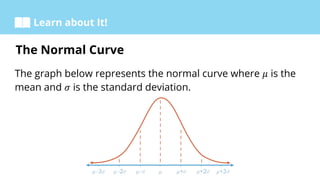
3. Objectives
At the end of this lesson, the learners should be able to
do the following:
● Construct a normal curve.
● Find the area of a region under the normal
curve.
● Solve real-life problems involving the normal
curve.

4. Learn about It!
The normal curve or bell curve is a graph that represents the
probability density function of the normal probability
distribution.
The normal curve is also called the Gaussian curve, named
after the mathematician Carl Friedrich Gauss.
The Normal Curve

5. Learn about It!
The graph below represents the normal curve where 𝜇 is the
mean and 𝜎 is the standard deviation.
The Normal Curve

6. Learn about It!
This rule states that the area of the region between one
standard deviation away from the mean is 0.6826, two
standard deviations away from the mean is 0.9544, and
three standard deviations away from the mean is 0.9974.
Empirical Rule

7. Learn about It!
Area of the Region between One Standard
Deviation Away from the Mean

8. Learn about It!
Area of the Region between Two Standard
Deviations Away from the Mean

9. Learn about It!
Area of the Region between Three Standard
Deviations Away from the Mean

10. Try it!
Let’s Practice
Example 1: What is the area of the scores in a normally
distributed data that is more than one standard deviation
above the mean?

11. Solution to Let’s Practice
Solution:
1. Shade the region in the normal curve that is more than
one standard deviation above the mean.
Example 1: What is the area of the scores in a normally distributed data that is more than
one standard deviation above the mean?

12. Solution to Let’s Practice
Solution:
2. Use the empirical rule to find the area of the given region.
Find the area of the region one standard deviation away from
the mean. By empirical rule, the area of this region is 0.6826.
The shaded area is shown on the next slide.
Example 1: What is the area of the scores in a normally distributed data that is more than
one standard deviation above the mean?

13. Solution to Let’s Practice
Solution:
2. Use the empirical rule to find the area of the given region.
Example 1: What is the area of the scores in a normally distributed data that is more than
one standard deviation above the mean?

14. Solution to Let’s Practice
Solution:
Since the normal curve is symmetric, we can obtain the area
of the region between the mean and one standard deviation
above the mean by dividing 0.6826 by 2.
To get the area of this region, divide 0.6826 by 2.
Example 1: What is the area of the scores in a normally distributed data that is more than
one standard deviation above the mean?

15. Solution to Let’s Practice
Solution:
0.6826 ÷ 2 = 0.3413
Example 1: What is the area of the scores in a normally distributed data that is more than
one standard deviation above the mean?

16. Solution to Let’s Practice
Solution:
To get the area of the region more than one standard
deviation above the mean, subtract 0.3413 from 0.5 since half
of the area of a normal curve is 0.5.
Example 1: What is the area of the scores in a normally distributed data that is more than
one standard deviation above the mean?

17. Solution to Let’s Practice
Solution:
0.5 − 0.3413 = 0.1587
Example 1: What is the area of the scores in a normally distributed data that is more than
one standard deviation above the mean?

18. Solution to Let’s Practice
Solution:
Thus, the area of the region more than one standard
deviation above the mean is 𝟎. 𝟏𝟓𝟖𝟕.
Example 1: What is the area of the scores in a normally distributed data that is more than
one standard deviation above the mean?

19. Try it!
Let’s Practice
Example 2: The mean and standard deviation of a normally
distributed scores are 15.8 and 2.2, respectively. Construct
the normal curve of the data.

20. Solution to Let’s Practice
Solution:
1. Solve for the scores one, two, and three standard
deviations away from the mean.
𝜇 = 15.8, 𝜎 = 2.2
Example 2: The mean and standard deviation of a normally distributed scores are 15.8 and
2.2, respectively. Construct the normal curve of the data.

21. Solution to Let’s Practice
Solution:
a. One standard deviation away from the mean
𝜇 + 𝜎 = 15.8 + 2.2
= 18
𝜇 − 𝜎 = 15.8 − 2.2
= 13.6
Example 2: The mean and standard deviation of a normally distributed scores are 15.8 and
2.2, respectively. Construct the normal curve of the data.

22. Solution to Let’s Practice
Solution:
b. Two standard deviations away from the mean
𝜇 + 2𝜎 = 15.8 + 2(2.2)
= 15.8 + 4.4
= 20.2
Example 2: The mean and standard deviation of a normally distributed scores are 15.8 and
2.2, respectively. Construct the normal curve of the data.

23. Solution to Let’s Practice
Solution:
b. Two standard deviations away from the mean
𝜇 − 2𝜎 = 15.8 − 2(2.2)
= 15.8 − 4.4
= 11.4
Example 2: The mean and standard deviation of a normally distributed scores are 15.8 and
2.2, respectively. Construct the normal curve of the data.

24. Solution to Let’s Practice
Solution:
c. Three standard deviations away from the mean
𝜇 + 3𝜎 = 15.8 + 3(2.2)
= 15.8 + 6.6
= 22.4
Example 2: The mean and standard deviation of a normally distributed scores are 15.8 and
2.2, respectively. Construct the normal curve of the data.

25. Solution to Let’s Practice
Solution:
c. Three standard deviations away from the mean
𝜇 − 3𝜎 = 15.8 − 3(2.2)
= 15.8 − 6.6
= 9.2
Example 2: The mean and standard deviation of a normally distributed scores are 15.8 and
2.2, respectively. Construct the normal curve of the data.

26. Solution to Let’s Practice
Solution:
2. Construct the normal curve using the set of scores
obtained from the previous step.
Using the mean as the center and the set of scores, we can
construct the normal curve as follows:
Example 2: The mean and standard deviation of a normally distributed scores are 15.8 and
2.2, respectively. Construct the normal curve of the data.

27. Solution to Let’s Practice
Solution:
Example 2: The mean and standard deviation of a normally distributed scores are 15.8 and
2.2, respectively. Construct the normal curve of the data.

28. Try It!
Individual Practice:
1. In a normally distributed data, find the area of the scores
less than two standard deviations below the mean.
2. Construct the normal curve of a given data with 𝜇 = 37.6
and 𝜎 = 3.9.

29. Try It!
Group Practice: To be done in groups of five.
Mr. Esguerra gave a 50-item test to his class and got a mean
score of 34.8 and a standard deviation of 1.5. Given that the
scores are normally distributed, what percent of the students
got 33.3 and below?

30. Key Points
● A normal curve or a bell curve is a graph that
represents the probability density function of a normal
probability distribution. It is also called a Gaussian
curve—named after the mathematician Carl Friedrich
Gauss.

31. Key Points
● The empirical rule states that the area of the region
between one standard deviation away from the mean is
0.6826, two standard deviations away from the mean is
0.9544, and three standard deviations away from the
mean is 0.9974.