Nonlinear Programming: Theories and Algorithms of Some Unconstrained Optimization Methods (Steepest Descent and Newton’s Method)

International Journal of Engineering and Management Research e-ISSN: 2250-0758 | p-ISSN: 2394-6962
Volume-10, Issue-2 (April 2020)
www.ijemr.net https://doi.org/10.31033/ijemr.10.2.1
1 This work is licensed under Creative Commons Attribution 4.0 International License.
Nonlinear Programming: Theories and Algorithms of Some
Unconstrained Optimization Methods
(Steepest Descent and Newton’s Method)
Onanaye, Adeniyi Samson
Senior Lecturer, Department of Mathematical Sciences, Industrial Mathematics Programme, Redeemer's University, NIGERIA
Corresponding Author: onanayea@run.edu.ng
ABSTRACT
Nonlinear programming problem (NPP) had become
an important branch of operations research, and it was the
mathematical programming with the objective function or
constraints being nonlinear functions. There were a variety of
traditional methods to solve nonlinear programming problems
such as bisection method, gradient projection method, the
penalty function method, feasible direction method, the
multiplier method. But these methods had their specific scope
and limitations, the objective function and constraint
conditions generally had continuous and differentiable
request. The traditional optimization methods were difficult to
adopt as the optimized object being more complicated.
However, in this paper, mathematical programming
techniques that are commonly used to extremize nonlinear
functions of single and multiple (n) design variables subject to
no constraints are been used to overcome the above challenge.
Although most structural optimization problems involve
constraints that bound the design space, study of the methods
of unconstrained optimization is important for several
reasons. Steepest Descent and Newton’s methods are employed
in this paper to solve an optimization problem.
Keywords-- Nonlinear Programming Problem,
Unconstrained Optimization, Mathematical Programming,
Newton's Method, Steepest Descent
2010 Mathematics Subject Classification: 12Y05
I. INTRODUCTION
Analysts of operations research, managers,
engineers of all kinds and planner faced by problems which
needs to be solve. These problems may imply arriving at an
optimal design, finding the flight of a jet etc. For example,
in the engineering design, because there was no continuity
in competition so therefore, it was communal to include a
large safety factor. Now that there is continuity in
competition, it is no longer capable to develop only an
acceptable design. In other instance, such as in engineering
motorcycle design, the development may be limited. Hence
we ask questions like: can we find a more economical
design? Are we making use of the scarce resources
effectively? Are we taking risk within the bankable limits?
In response to all these, there has been a very rapid growth
of optimization techniques and models.
The acceptance of the field of operations research
in the study of business, and industrial activities can be
attributed, at least in part, to the extent to which the
operations research methods and approach have aided the
decision makers. The application of operations research in
the early post-war was mainly in the area of linear
programming and use of statistics. Linear programming
(LP) is used to find the most accurate outcomes (such as
minimum cost or maximum profit) in a mathematical model
whose requirements are imaged by linear relationships.
Linear programming and nonlinear programming (NLP) are
both similar in that it is compose of an objective function,
general constraint, and (NLP) includes at least one
nonlinear function, which could be the objective function,
or some or all of the constraints.
Many real systems are inherently nonlinear, for
example: the fall in signal strength or power with distance
from the transceiver (antenna), so therefore, it is important
that optimization algorithms be able to handle them.
In mathematics, nonlinear programming (NLP) is
the process of solving an optimization problem defined by a
system of equalities and inequalities, collectively termed
constraints, over a set of unknown real variables, along with
an objective function to be maximized or minimized, where
some of the constraints or the objective function are
nonlinear. It is the sub-field of Mathematical optimization
that deals with problems that are not linear. (Wikipedia.).
However, in this paper, unconstrained optimization is been
considered and discussed.
1.1 Statement of the Problem
In time past, engineers, operations researchers,
managers, etc were faced with problems to be solved. Some
of these problems can be modelled into mathematical
functions or equations which might not be linear (nonlinear
systems of equations) and may be subject to some
constraints or no constraints (unconstraint). Nonlinear
programming approach can be employed to solve such
mathematical equations. Here, we are looking at problems
that involve nonlinear equations that are not subjected to

constraints by applying two unconstraint optimization
methods, Steepest Descent method and Newton’s method
and compare results.
1.2 Aim and Objective
Aim of the Study
 The aim is to solve unconstrained optimization
problem using Steepest Descent and Newton’s
method and comparing the behaviour of their
result in terms of rate of convergence and degree
of accuracy.
Objectives of the Study
 The objective is to do a proper study of
unconstrained optimization problem studying two
methods which is Steepest Descent and Newton’s
method
 To solve an example using the two methods and
compare the results
1.3 Significance of the Study
Unconstrained optimization is important for the
following reasons:
 If the design is at a stage where no constraints are
active then the process of determining a search
direction and travel distance for minimizing the
objective function involves an unconstrained
function minimization algorithm. Of, course in
such a case one has constantly to watch for
constraint violations during the move in design
space.
 A constrained optimization problem can be cast as
an unconstrained minimization problem even if the
constraints are active.
 Unconstrained minimization strategies are
becoming increasingly popular as techniques
suitable for linear and nonlinear structural analysis
problems which involve solution of a system of
linear or nonlinear equations.
1.4 Limitations of the Study
The problem in nonlinear programming is that
nonlinear models are much more difficult to optimize.
Some of the problems are listed below:
 Numerical methods for solving nonlinear
programs have limited information about the
current point.
 Different algorithms and methods arrive at
different solutions and outcome.
 Different but equivalent formulations of the model
given to the same solver may produce different
solution and outcomes.
 Different starting point may lead to different final
solution.
 It may be difficult to find a feasible starting point.
 There is no finite determination of the outcome.
 It is difficult to determine whether the conditions
to apply a particular method are met.(Chinneck,
2012)
1.5 Definition of Some Terms
Unconstrained optimization: Unconstrained
optimization is an optimization that is subject to no
constraints. Such problems may contain one or N variables.
Univariate: Problems with a single variable are
called univariate. The univariate optimum for
occurs at points where the first derivative of with
respect to equals zero. However, points which
have zero first derivatives do not necessarily constitute a
minimum or maximum. The second derivative is used to
discover character of a point. Points at which a relative
minimum occurs have a positive second derivative at that
point while relative maximum occurs at points with a
negative second derivative. Zero second derivatives are
inconclusive.
It is important to distinguish between local and
global optima. A local optimum arises when one finds a
point whose value in the case of a maximum exceeds that of
all surrounding points but may not exceed that of distant
points. The second derivative indicates the shape of
functions and is useful in indicating whether the optimum is
local or global. The second derivative is the rate of change
in the first derivative. If the second derivative is always
negative (positive) that implies that any maximum
(minimum) found is a global result. Consider a
maximization problem with a negative second derivative
for which . This means the first derivative was >
0 for and was < 0 for . The function can
never rise when moving away from X* because of the sign
of the second derivative. An everywhere positive second
derivative indicates a global minimum will be found
if , while a negative indicates a global
maximum.
Multivariate functions: The univariate
optimization results have multivariate analogues. In the
multivariate case, partial derivatives are used, and a set of
simultaneous conditions is established. The first and second
derivatives are again key to the optimization process,
excepting now that a vector of first derivatives and a matrix
of second derivatives is involved.
There are several terms to review. First, the gradient vector,
, is the vector of first order partial derivatives of a
multivariate function with respect to each of the variables
evaluated at the point .
(1.0)
where;

Stands for the partial derivative of f(X) with
respect to Xj. The second derivatives constitute the Hessian
matrix,
(1.1)
The Hessian matrix, evaluated is an N by N
symmetric matrix of second derivatives of the function with
respect to each variable pair.
The multivariate version of the second derivative
test involves examination of the Hessian matrix. If the
Hessian matrix is neither positive nor negative definite,
then no conclusion can be made about whether this point is
a maximum or minimum and one must conclude it is an
inflection or saddle point.( McCarl, 2010).
II. NONLINEAR PROGRAMMING
The paper that first used the name ‘nonlinear
programming’ was written 41 years ago.
In the intervening period, there were a number of
things about the influences, both mathematical and social,
that have shaped the modern development of the subject.
Some of these are quite old and long predate the
differentiation of nonlinear programming as a separate area
for research. Others are comparatively modern and
culminate in the period 41 years ago when this
differentiation took place.Tucker, (1997).
2.1 Basic Concepts of Optimization Methods
Optimization problems can be classified based on
the type of constraints, nature of design variables, physical
structure of the problem, nature of the equations involved,
deterministic nature of the variables, permissible value of
the design variables, separability of the functions and
number of objective functions. These classifications are
briefly discussed below.
2.1.1 Classification Based on Existence of Constraints
Under this category optimizations problems can be
classified into two groups as follows:
Constrained Optimization Problems: which are subject to
one or more constraints.
Unconstrained Optimization Problems: in which no
constraints exist.
2.1.2 Classification Based on the Nature of the Design
Variables
There are two broad categories in this
classification.
(i) In the first category the objective is to find a set
of design parameters that makes a prescribed function of
these parameters minimum or maximum subject to certain
constraints. For example to find the minimum weight
design of a strip footing with two loads shown in Fig 1 (a)
subject to a limitation on the maximum settlement of the
structure can be stated as follows.
Find X = which minimizes (2.0)
f(X) = h(b,d)(2.1)
Subject to the constraints X ) ; b 0
; d 0 (2.1.1)
where is the settlement of the footing. Such problems
are called parameter or static optimization problems.
It may be noted that, for this particular example,
the length of the footing (l), the loads P1 and P2 and the
distance between the loads are assumed to be constant and
the required optimization is achieved by varying b and d.
(Kumar, 2014).
(ii) In the second category of problems, the
objective is to find a set of design parameters, which are all
continuous functions of some other parameter that
minimizes an objective function subject to a set of
constraints. If the cross sectional dimensions of the
rectangular footings are allowed to vary along its length as
shown in Fig 3.1 (b), the optimization problem can be
stated as :
Find X(t) = which minimizes (2.2)
f(X) = g( b(t), d(t) ) (2.3)
Subject to the constraints
X(t)) 0 t l (2.3.1)
b(t) 0 0 t l (2.4)
d(t) 0 0 t l (2.5)
The length of the footing (l) the loads P1 and P2 ,
the distance between the loads are assumed to be constant
and the required optimization is achieved by varying b and
d along the length l. ( Kumar2014).
Here the design variables are functions of the
length parameter t. this type of problem, where each design
variable is a function of one or more parameters, is known
as trajectory or dynamic optimization problem.






d
b
(s max 

s






)(
)(
td
tb
(s max  
  
  

Figure 1 (a) Figure 1 (b)
2.1.3 Classification Based on the Physical Structure of the
Problem
Based on the physical structure, optimization
problems are classified as optimal control and non-optimal
control problems.
(i) Optimal Control Problems
An optimal control (OC) problem is a
mathematical programming problem involving a number of
stages, where each stage evolves from the preceding stage
in a prescribed manner. It is defined by two types of
variables: the control or design and state variables. The
control variables define the system and controls how one
stage evolves into the next. The state variables describe the
behavior or status of the system at any stage. The problem
is to find a set of control variables such that the total
objective function (also known as the performance index,
PI) over all stages is minimized, subject to a set of
constraints on the control and state variables. An OC
problem can be stated as follows:
FindX which minimizes f(X) = (2.6)
i = 1, 2…l (2.6.1)
, j = 1, 2…l (2.6.2)
, k = 1, 2…l (2.6.3)
Where xi is the ith control variable, yi is the ith
state variable, and fi is the contribution of the ith stage to
the total objective function. gj, hk, and qi are the functions
ofxj, yj ;xk, yk and xi andyi, respectively, and l is the total
number of states. The control and state variables xi andyi
can be vectors in some cases.
(ii) Problems which are not optimal control problems are
called non-optimal control problems.
2.1.4 Classification Based on the Nature of the Equations
Involved
Based on the nature of equations for the objective
function and the constraints, optimization problems can be
classified as linear, nonlinear, geometric and quadratic
programming problems. The classification is very useful
from a computational point of view since many predefined
special methods are available for effective solution of a
particular type of problem.
(i) Linear Programming Problem
If the objective function and all the constraints are
‘linear’ functions of the design variables, the optimization
problem is called a linear programming problem (LPP). A
linear programming problem is often stated in the standard
form:
),(
1
ii
l
i
i yxf
1),(  iiiii yyyxq
0)( jj xg
0)( kk yh
l l
P1
P2
d
b
P2
P1
b(t)
d(t)
t

Find X = (2.7)
Which maximizes f(X) = (2.7.1)
, j = 1, 2, . . . ,m (2.7.2)
xi , j = 1, 2, . . . , m (2.7.3)
where
ci, aij, and bj are constants.
(ii) Nonlinear Programming Problem
If any of the functions among the objectives and
constraint functions is nonlinear, the problem is called a
nonlinear programming (NLP) problem. This is the most
general form of a programming problem and all other
problems can be considered as special cases of the NLP
problem.
(iii) Geometric Programming Problem
A geometric programming (GMP) problem is one
in which the objective function and constraints are
expressed as polynomials in X. A function h(X) is called
apolynomial (with terms) if h can be expressed as
(2.8)
where
cj ( ) and aij ( and ) are constants with and Thus GMP problems can
be posed as follows:
Find X which minimizes
f(X) = cj> 0, xi> 0 (2.9)
subject to
gk(X) = ajk> 0, xi> 0, k = 1,2,…..,m (2.9.1)
whereN0 and Nk denote the number of terms in the
objective function and in the kth
constraint function,
respectively.
(iv) Quadratic Programming Problem
A quadratic programming problem is the best
behaved nonlinear programming problem with a quadratic
objective function and linear constraints and is concave (for
maximization problems). It can be solved by suitably
modifying the linear programming techniques. It is usually
formulated as follows:
F(X) = (2.10)
Subject to
















nx
x
x
.
.
2
1
i
n
i
i xc1
ji
n
i
ij bxa 1
0
m
mj ,,1  ni ,,1  mj ,,1  0jc 0ix
,
0
1 1
 





N
j
n
i
ija
ij xc 
,0
1 1
 





kN
j
n
i
ijkq
ijk xa 
  

n
i
n
j
jiij
n
i
ii xxQxqc
1 11

j = 1,2,….,m
xi , i = 1,2,….,n
where
c, qi, Qij, aij, and bj are constants.
2.1.5 Classification Based on the Permissible Values of
the Decision Variables
Under this classification, objective functions can
be classified as integer and real-valued programming
problems.
(i) Integer Programming Problem
If some or all of the design variables of an
optimization problem are restricted to take only integer (or
discrete) values, the problem is called an integer
programming problem. For example, the optimization is to
find number of articles needed for an operation with least
effort. Thus, minimization of the effort required for the
operation being the objective, the decision variables, i.e. the
number of articles used can take only integer values. Other
restrictions on minimum and maximum number of usable
resources may be imposed.
(ii) Real-Valued Programming Problem
A real-valued problem is that in which it is sought
to minimize or maximize a real function by systematically
choosing the values of real variables from within an
allowed set. When the allowed set contains only real values,
it is called a real-valued programming problem.
2.1.6 Classification Based on Deterministic Nature of the
Variables
Under this classification, optimization problems
can be classified as deterministic or stochastic
programming problems.
(i) Stochastic Programming Problem
In this type of an optimization problem, some or
all the design variables are expressed probabilistically (non-
deterministic or stochastic). For example estimates of life
span of structures which have probabilistic inputs of the
concrete strength and load capacity is a stochastic
programming problem as one can only estimate
stochastically the life span of the structure.
(ii) Deterministic Programming Problem
In this type of problems all the design variables
are deterministic.
2.1.7 Classification Based on Separability of the
Functions
Based on this classification, optimization
problems can be classified as separable and non-separable
programming problems based on the separability of the
objective and constraint functions.
(i) Separable Programming Problems
In this type of a problem the objective function
and the constraints are separable. A function is said to be
separable if it can be expressed as the sum of n single-
variable functions,
, i.e.
(2.11)
and separable programming problem can be expressed in standard form as :
Find X which
minimizes (2.12)
subject to
, j = 1,2,. . . , m (2.12.1)
where
bj is a constant.
0
     nni xfxfxf ,..., 221
 

n
i
ii xfXf
1
)(
 

n
i
ii xfXf
1
)(
  j
n
i
iijj bxgXg  1
)(

2.1.8 Classification Based on the Number of Objective
Functions
Under this classification, objective functions can
be classified as single-objective and multi-objective
programming problems.
(i) Single-Objective Programming Problem in which
there is only a single objective function.
(ii) Multi-Objective Programming Problem
A multi-objective programming problem can be stated as
follows:
Find X which minimizes (2.13)
Subject to
gj(X) , j = 1, 2, . . . , m
wheref1, f2 . . . fk denote the objective functions to be minimized simultaneously.
For example in some design problems one might
have to minimize the cost and weight of the structural
member for economy and, at the same time, maximize the
load carrying capacity under the given constraints.
(Kumar,2014).
III. METHODOLOGY
Methodology is the systematic, theoretical analysis
of the methods applied to a field of study. It comprises the
theoretical analysis of the body of methods and principles
associated with a branch of knowledge. Typically, it
encompasses concepts such as paradigm, theoretical model,
phases and quantitative or qualitative techniques. Note that
a methodology does not set out to provide solutions to the
problem
3.1 Steepest Descent Method
This method is also known as conjugate direction
method.
Move in the direction of steepest ascent. Compute the slope
of the function at the local point. From this obtain the best
direction to move. Hill Climbing scheme.
Figure 2(a)
At next iteration,
Figure 2(b)
     XfXfXf k,..., 21
0

And, again at next iteration,
Figure 2(c)
Looking into the process from the beginning till the ascent is complete; it looks like the following on a contour plot
Figure 3
3.2 Steepest Descent Algorithm
Choose a starting point kx . Find the local
gradient of the function at this point, i.e. obtain
kx
f .
Move in the direction of the gradient and select the next
evaluation point to be
kxkk fxx  1 (3.0)
Obtain  that maximizes )( 1kxf . Continue
the process till convergence is realized. This is Hill
climbing scheme. The above algorithm is for a multivariate
function.
To minimize a univariate function by Steepest Descent
Method, we start at some point and at k update the
algorithm of the Steepest Descent Method for a univariate
function is given below:
(3.1)
where and is regarded as the step size.
A wrong step size may not reach convergence,
so a careful selection of the step size is important. Too large
will diverge; too small it will take long a long time to
converge. The best way is to choose a fixed step size that
will assure convergence wherever you start Steepest
Descent.
Now, the formula for the Steepest Descent Method in this
case is:

(3.2)
3.3 Newton’s Method
Newton’s method is a general procedure that can
be applied in many diverse situations. When specialized to
the problem of locating a zero of real-valued function of a
real variable, it is often called Newton-Raphson iteration. In
general, Newton’s method is faster than the bisection
method and Fixed-Point iteration since its convergence is
quadratic rather than linear. Once the quadratic becomes
effective, that is, the values of Newton’s method sequence
are sufficiently close to the root, the convergence is so rapid
that only a few more values are needed. Unfortunately, the
method is not guaranteed always to convergence. Newton’s
method is often combined with other slower method in a
hybrid method that is numerically globally convergence.
Suppose that we have a function f whose zeros are to be
determined numerically. Let r be a zero of )(xf and let
x be an approximation to r . If f  exists and is
continuous, then by Taylor’s Theorem,
         2
0 hoxfhxfhxfrf  , (3.3)
Where xrh  . If h is small (that is, x is near r ), then it is reasonable to ignore the  2
ho term and solve the remaining
equation for h . If we do this, the result is    xfxfh  . If x is an approximation to r , then    xfxfx  should
be r . Newton’s method begins with an estimate 0x of r and then defines inductively
xn+1 = xn -
f (xn )
¢f xn( )
n ³ 0( ). (3.4)
3.3.1 Newton’s Algorithm
x0 = Initial guess
xn+1 = xn -
f (xn )
¢f xn( )
, for n = 0,1,2, (3.5)
Before examining the theoretical basis for
Newton’s method, let’s give a graphical interpretation of it.
From the description already given, we can say that
Newton’s method involves linearizing the function. That is,
f was replaced by a linear function. The usual way of
doing this is to replace f by the first two terms in the
Taylor series. Thus, if
          
2
!2
1
cxcfcxcfcfxf . (3.6)
Then the linearization (at c) produces the linear function
      cxcfcfxl  . (3.7)
Note that l is a good approximation to f in the
vicinity of c , and in fact we have    cfcl  and
   cfcl  . Thus, the linear function has the same value
and the same slope as fit the point c . So in Newton’s
method we are constructing the target line to f at a point
near r , and finding where the target line intersects the x -
axis.
IV. DATA PRESENTATION ANANLYSIS
AND INTERPRETATION
4.1 Minimization of the Optimization Problem
In this section, there will be a comparison between
the two unconstrained optimization methods. We use the
two methods to solve an optimization problem. As we
know, the two unconstrained optimization methods to be
used to solve the optimization problem are Steepest Descent
Method and Newton’s Method.
The optimization problem to be solved is a univariate
function. The function to be optimized will be minimized is
given below:
(4.0)

4.2 Steepest Descent Method
Using the Steepest Descent method to solve the
above function, we are going to use the formula for
univariate functions which is:
(4.1)
where , therefore (4.2)
The derivative of is easily computed:
(4.3)
Then we need to choose an initial point for =10 and
When then,
= 9.14195
Therefore,
Since and 0.858050,
we continue to iterate by substituting to the Steepest
Descent formula as to obtain and so
on until we get to the iterate at which it converges. The
complete iteration sequence is given in the table below:
4.2.1 Iterates of Steepest Descent Method
0 10.00000 0.858050 9.141950
1 9.141950 0.700741 8.441209
2 8441209 0.584069 7.857140
3 7.857140 0.494927 7.362213
4 7.362213 0.425158 6.937055
5 6.937055 0.369448 6.567607
6 6.567607 0.324209 6.243398
7 6.243398 0.286939 5.956459
8 5.956459 0.255846 5.700613
9 5.700613 0.229623 5.470990
10 5.47099 0.207292 5.263698
11 5.263698 0.188109 5.075589
12 5.075589 0.167105 4.908484
13 4.908484 0.157398 4.751086
14 4.751086 0.144661 4.606425

15 4.606425 0.133426 4.472999
16 4.472999 0.123465 4.349534
17 4.349534 0.114590 4.234944
18 4.234944 0.106648 4.128296
19 4.1288296 1.064130 3.064166
20 3.064166 1.053321 2.010845
21 2.010845 0.008666 2.002179
22 2.002179 0.008325 1.993686
23 1.993686 0.008325 1.985361
24 1.985361 0.008113 1.9772480
25 1.977248 0.008005 1.969243
26 1.969243 0.007851 1.961392
27 1.961255 0.007691 1.96034
Source: Research field study, 2019
The Steepest Descent method converges to
at the 27th
iteration.
4.3 Newton’s Method
Using the univariate formula of Newton’s method
to solve the optimization problem that was solved using
Steepest Descent method.
(4.4)
Thus, algorithm make progression as long as
.The algorithm above determines its next
estimate.
Now, we consider the function to be minimized:
(4.5)
is also known as the derivative of which is:
(4.6)
Let’s now assume an initial point
When then,
The value for and
2.978923. As discussed in Steepest Descent method,
we continue to iterate by substituting to the Newton’s
formula as to obtain and so on until
we get to the rate at which it converges. The complete
iteration sequence is given in the table below:
4.3.1 The iterates of Newton’s Method
0 10.000000 2.978923 7.0321080
1 7.0321080 1.976429 5.055679
2 5.055679 1.314367 3.741312
3 3.741312 0.871358 2.869995
4 2.869995 0.573547 2.296405
5 2.296405 0.371252 1.925154

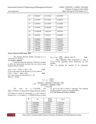
6 1.925154 0.230702 1.694452
7 1.694452 0.128999 1.565453
8 1.565453 0.054156 1.511296
9 1.511296 0.0108640 1.500432
10 1.500432 0.000431 1.500001
Source: Research field study, 2019
After the iteration, our convergence to at
the 5th
iteration.
Now considering the iteration s of the two
methods, we noticed that the rate at which Steepest Descent
uses to converge is slow because it was at the 27th
iterate it
got its convergence. While for Newton’s the rate of
convergence is fast in the sense that it converged at the 10th
iteration and it is more accurate.
Previous researchers have also concluded that
Newton’s method is faster and more accurate than other
optimization methods.
V. CONCLUTION
In this work, the researchers tried to examine the
rate at which the two unconstrained optimization method
will converge and the accuracy of the methods.
The objective of this research work is to find out
which method is more accurate to getting to the
convergence point. It was observed that the Steepest
Descent method took a longer time before it got to the point
of convergence while for that of Newton’s method, the rate
at which it got to the point of convergence was far faster
and more accurate than Steepest Descent method.
This paper work was aimed at studying the
convergence of two unconstrained optimization methods
using the two methods to solve the same optimization
problem. It highlights the significance of the study,
limitations and definition of some terms, which formed the
parameters for the research to work with. It also focuses on
the basics of optimization methods, types of problem and
what method could be used in solving them. The two
unconstrained optimization methods chosen were used to
solve an optimization method, checking their convergence
point and their rate of convergence.
5.1 Recommendation
1. It is recommended that Newton’s method should
be used preferred to Steepest Descent method for
easy computation and accurate solution.
2. There should be a fixed value for the step size in
Steepest Descent method.
3. This project work is recommended to those
interested in carrying out optimization subject to
no constraint. The right method should be used
depending on the problem definition and target
goal.
REFERENCES
[1] Charnes .A. & Cooper W.W. (1962). ’Programming
with linear fractional functional. Available at:
https://onlinelibrary.wiley.com/doi/abs/10.1002/nav.380010
0123.
[2] Bradley S.P. & Frey S.C. (1974). Fractional
programming with homogeneous functions. Operations
Research, 22(2), 350-357.
[3] Dr. Binay Kuma. (2014). Advanced method for solution
of constraint optimization problems. Available at:
https://rd.springer.com/book/10.1007%2F978-981-13-
8196-6.
[4] Holt C. C, Modigliani F, Muth J. F, & Simon H. A.
(1960). Planning production, inventories, and work-force,
New Jersey: Prentice-Hall, Inc.
[5] John W. Chinneck. (2012). Practical optimization: A
gentle introduction. Available at:
http://www.sce.carleton.ca/faculty/chinneck/po.html.
[6] Kuhn, H. & A. Tucker. (1950). Nonlinear
programming. Available at:
http://web.math.ku.dk/~moller/undervisning/MASO2010/k
uhntucker1950.pdf.
[7] Slater M. (1950). Lagrange multipliers revisited: A
contribution to nonlinear programming. Available at:
https://cowles.yale.edu/sites/default/files/files/pub/cdp/m-
0403.pdf.
[8] White L. S. (2018). ’Mathematical programming
models for determining freshman scholarship offers.
Forgotten Books.
[9] Winters P. R. (1962). Constrained inventory rules for
production smoothing. Management Science, 8(4).
[10] Van SlykeR. M. & Wets R. J. (1968). A duality theory
for abstract mathematical programs with applications to
optimal control theory. Available at:
https://apps.dtic.mil/docs/citations/AD0663661.

Nonlinear Programming: Theories and Algorithms of Some Unconstrained Optimization Methods (Steepest Descent and Newton’s Method)

Recommended

Recommended

More Related Content

What's hot

What's hot (20)

Similar to Nonlinear Programming: Theories and Algorithms of Some Unconstrained Optimization Methods (Steepest Descent and Newton’s Method)

Similar to Nonlinear Programming: Theories and Algorithms of Some Unconstrained Optimization Methods (Steepest Descent and Newton’s Method) (20)

More from Dr. Amarjeet Singh

More from Dr. Amarjeet Singh (20)

Recently uploaded

Recently uploaded (20)

Nonlinear Programming: Theories and Algorithms of Some Unconstrained Optimization Methods (Steepest Descent and Newton’s Method)