Downloaded 22 times


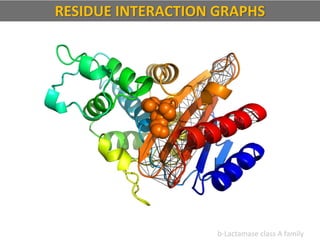
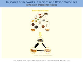
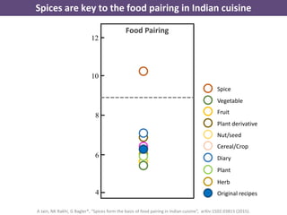
![Shikha Vashisht and Ganesh Bagler*, 7(11): e49401, PLoS ONE (2012). arXiv:1112.1510v2 [q-bio.MN]
Vinay Randhawa and Ganesh Bagler*, OMICS: A Journal of Integrative Biology, 16 (10) , 2012.
V Randhawa, P Sharma, S Bhushan and G Bagler*, OMICS: A Journal of Integrative Biology, 17(6), 302-317 (2013).
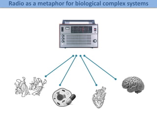
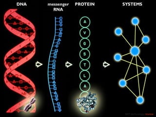
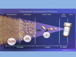
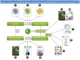
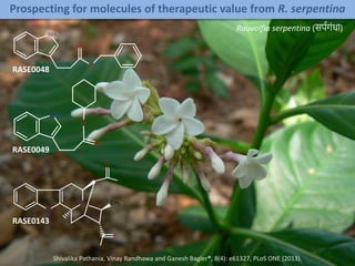
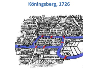
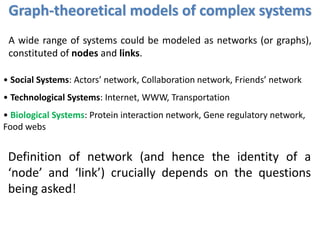
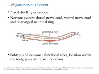
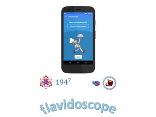
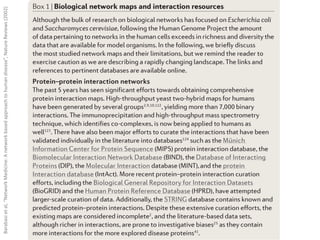
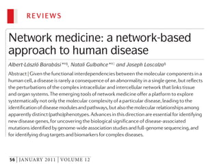
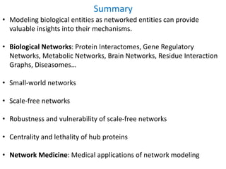
A rational approach towards ‘complex diseases’.
Data: KEGG, OMIM, PubMed, protein interactomes, gene regulations, expression data.
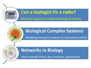
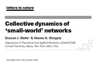
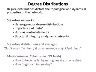
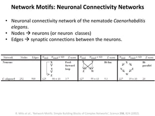
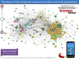
Network Models of Complex Diseases
Molecular interactomes of diseases phenotypes: Modeling and control
Why
What
How
model
Interactomes,
Expression data
control
targets, drugs](https://image.slidesharecdn.com/networksinbiosystemsdibrugarhgbagler-180107033126/85/Network-Biology-A-paradigm-for-modeling-biological-complex-systems-27-320.jpg)
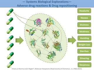
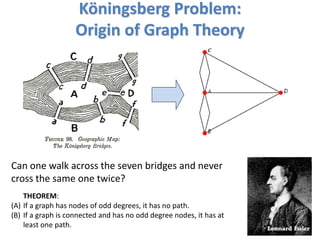
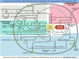
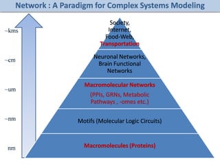
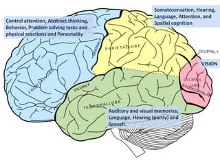
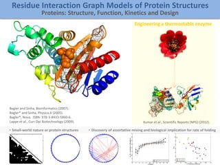
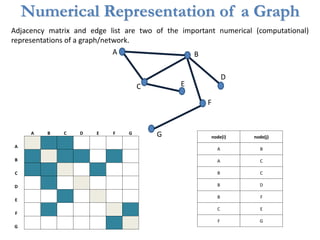
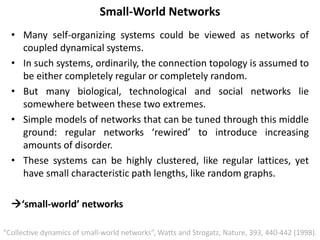
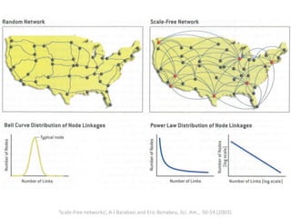
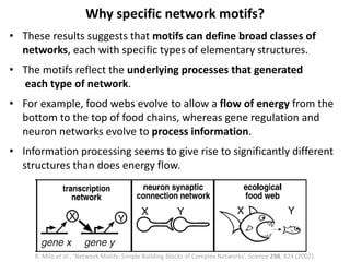
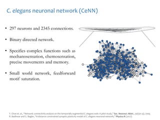
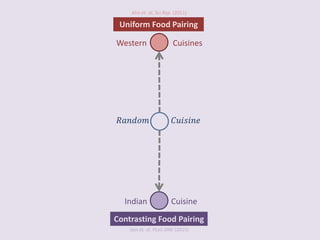
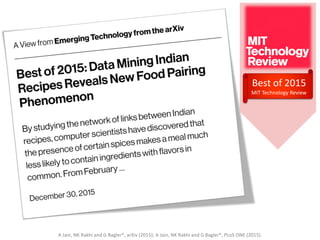
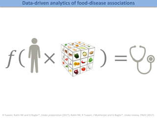
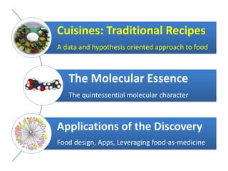
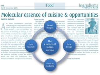
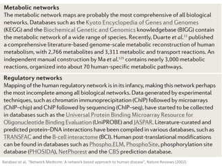
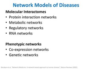
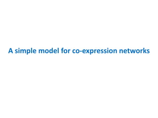
![Modeling a complex system as a graph
Undirected Network Directed Network
[DEFN] Degree: Number of nodes connected to a given node.
A
B
C
D
E
F G
A
B
C
D
E
F G
k_A=2; k_B=3 k_A_in=1; k_A_out=1;
k_B_in=3; k_B_in=1;
Weighted and Un-weighted Networks](https://image.slidesharecdn.com/networksinbiosystemsdibrugarhgbagler-180107033126/85/Network-Biology-A-paradigm-for-modeling-biological-complex-systems-37-320.jpg)
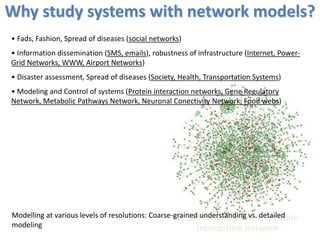


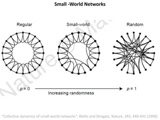


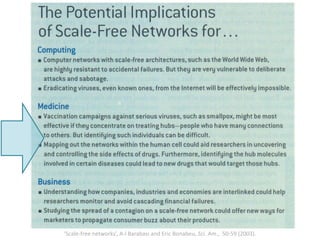
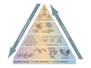
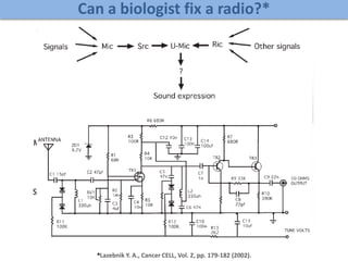
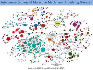
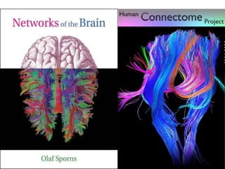
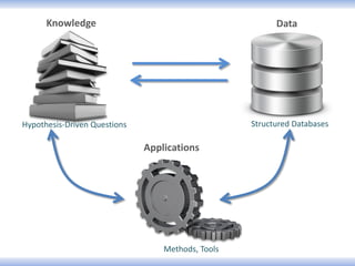
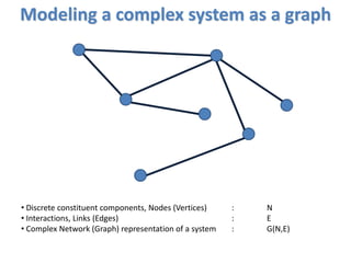
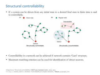
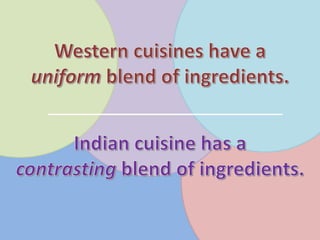
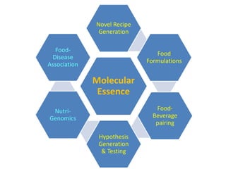
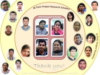
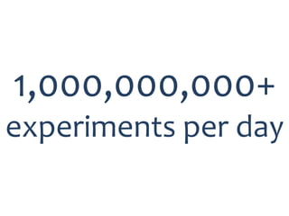
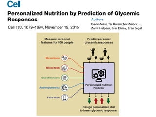
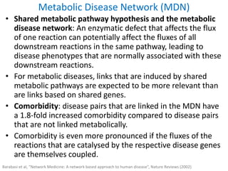
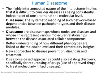
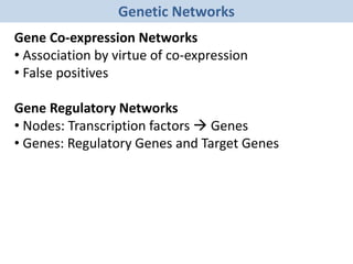
![Identification of Generic Cancer Genes: Cancer Genes Network (CGN)
Shikha Vashisht and Ganesh Bagler*, 7(11): e49401, PLoS ONE (2012). arXiv:1112.1510v2 [q-bio.MN]
• A protein interactome of interactions among cancer genes: Cancer Genes Network (CGN).
• Databases: CancerGenes Database, Human Protein Reference Database, KEGG-PIC.
• Central genes were identified using ‘degree’, ‘betweenness’ and ‘stress’ metrics.
11602 interactions
among 2665
cancer proteins](https://image.slidesharecdn.com/networksinbiosystemsdibrugarhgbagler-180107033126/85/Network-Biology-A-paradigm-for-modeling-biological-complex-systems-78-320.jpg)
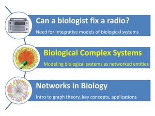
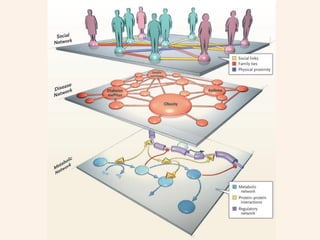
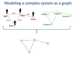
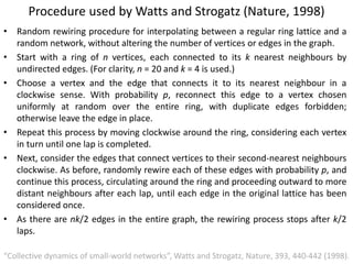
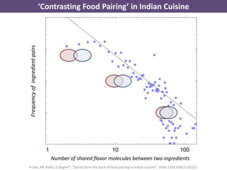
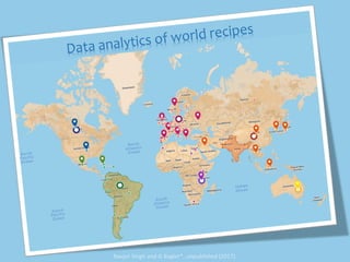
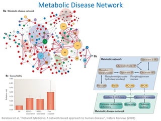
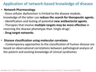
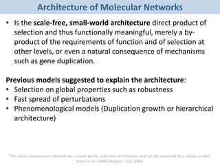
![Cancer Genes Network : Generic and Specific Cancer Genes
Shikha Vashisht and Ganesh Bagler*, 7(11): e49401, PLoS ONE (2012). arXiv:1112.1510v2 [q-bio.MN]
11602 interactions
among 2665
cancer proteins](https://image.slidesharecdn.com/networksinbiosystemsdibrugarhgbagler-180107033126/85/Network-Biology-A-paradigm-for-modeling-biological-complex-systems-79-320.jpg)
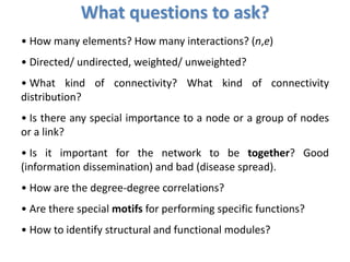
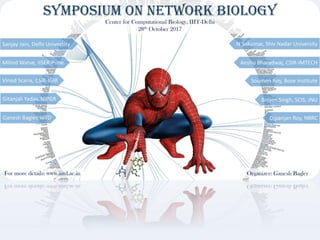
![● % Overlap of Central Genes in
‘Cancer Genes Network’ with
‘KEGG Pathways-in-Cancer’
Random Samplings
Negative Controls
The hubs and bottlenecks of ‘Cancer Genes Network’ represent
genes that are involved in generic cancer mechanisms.
Genes Central to ‘Cancer Genes Network’ match with KEGG-PIC
Shikha Vashisht and Ganesh Bagler*, 7(11): e49401, PLoS ONE (2012). arXiv:1112.1510v2 [q-bio.MN]](https://image.slidesharecdn.com/networksinbiosystemsdibrugarhgbagler-180107033126/85/Network-Biology-A-paradigm-for-modeling-biological-complex-systems-80-320.jpg)
![Hub Genes Random Samplings
1,2,3: Degree, Betweenness, Stress
4,5: Neighborhood connectivity,
Topological coefficient
6,7 (data not shown): Clustering coeff.,
Average shortest path length
Around 50% of a total 2665 cancer
genes of CGN, were ‘essential (1315)’.
Mouse Genome Informatics (MGI)
Phenotype Data.
Hubs of Cancer Genes Network (CGN) are ‘Biologically Essential’
Shikha Vashisht and Ganesh Bagler*, 7(11): e49401, PLoS ONE (2012). arXiv:1112.1510v2 [q-bio.MN]](https://image.slidesharecdn.com/networksinbiosystemsdibrugarhgbagler-180107033126/85/Network-Biology-A-paradigm-for-modeling-biological-complex-systems-81-320.jpg)
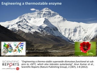
![Strategy for Identification of Targets Specific to Secondary Bone Cancer
Shikha Vashisht and Ganesh Bagler*, 7(11): e49401, PLoS ONE (2012). arXiv:1112.1510v2 [q-bio.MN]](https://image.slidesharecdn.com/networksinbiosystemsdibrugarhgbagler-180107033126/85/Network-Biology-A-paradigm-for-modeling-biological-complex-systems-82-320.jpg)
![(A) (B)
(C)
Subsets comprising
targets specific to
‘Secondary Bone
Cancer’
Identification of Targets Specific to Secondary Bone Cancer
Shikha Vashisht and Ganesh Bagler*, 7(11): e49401, PLoS ONE (2012). arXiv:1112.1510v2 [q-bio.MN]](https://image.slidesharecdn.com/networksinbiosystemsdibrugarhgbagler-180107033126/85/Network-Biology-A-paradigm-for-modeling-biological-complex-systems-83-320.jpg)
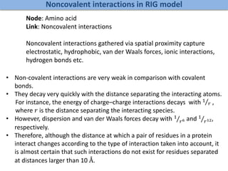
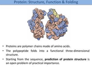
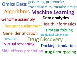
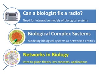
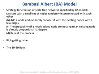
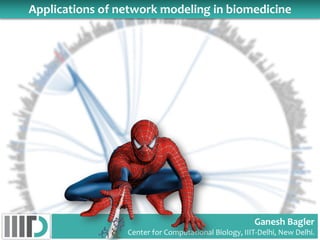
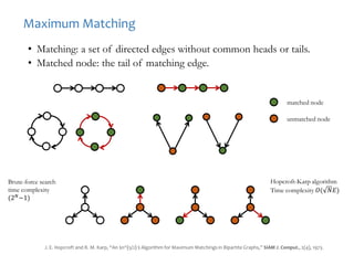
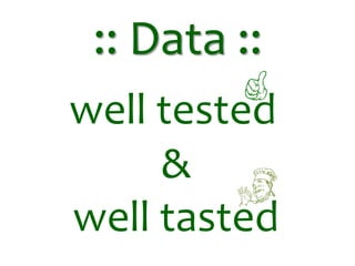
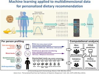
![Folding
Time
kF [sec-1]ln (kF)
7.389 s0.1353-2
1 s1.000
0.1353 s7.392
18.32 ms54.604
2.479 ms403.436
33.55 ms2,981.008
0.4540 s22,026.0010
6.144 s16275.4712
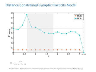
RATE OF FOLDING—FOLDING TIME
Bagler and Sinha, Bioinformatics (2007)](https://image.slidesharecdn.com/networksinbiosystemsdibrugarhgbagler-180107033126/85/Network-Biology-A-paradigm-for-modeling-biological-complex-systems-98-320.jpg)
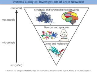
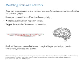
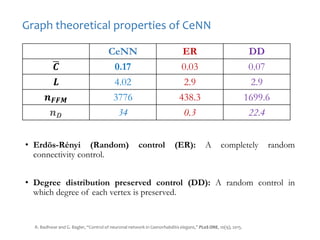


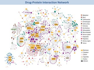
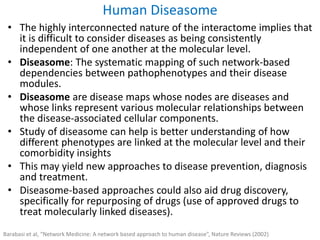
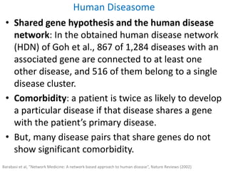
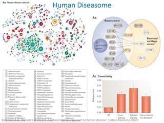


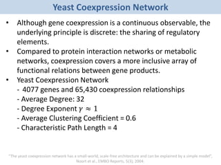
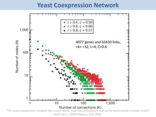


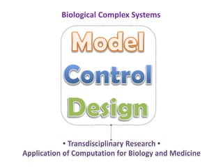
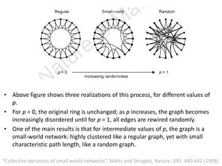
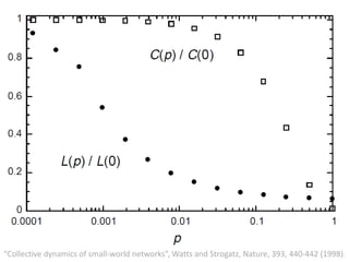
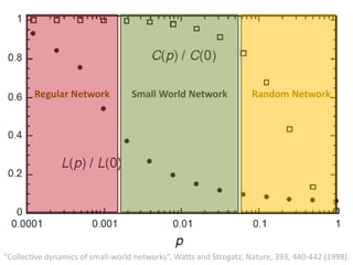
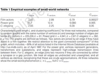
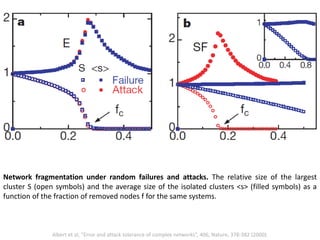
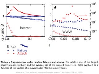
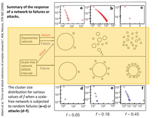
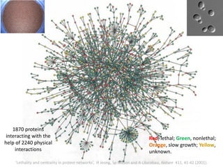
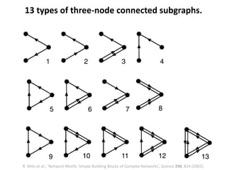
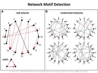
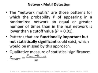
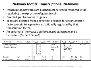
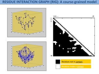
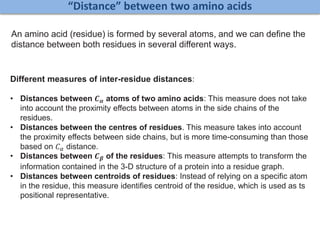
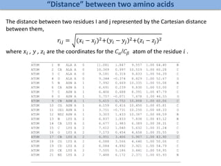
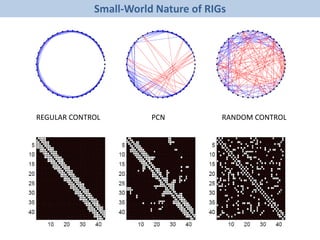
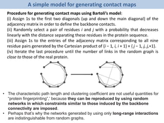
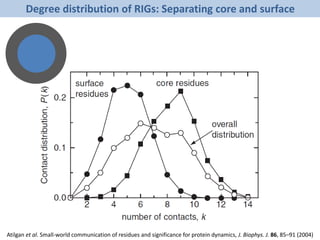
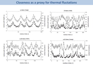
The document discusses network biology as a framework for modeling complex biological systems, emphasizing the importance of understanding biological entities as interconnected networks. It highlights various applications such as protein structure prediction, gene identification, and disease modeling through graph theory and network models. Additionally, it explores concepts like small-world networks, scale-free networks, and network motifs, along with their implications for biomedical research and the importance of integrative models in biology.