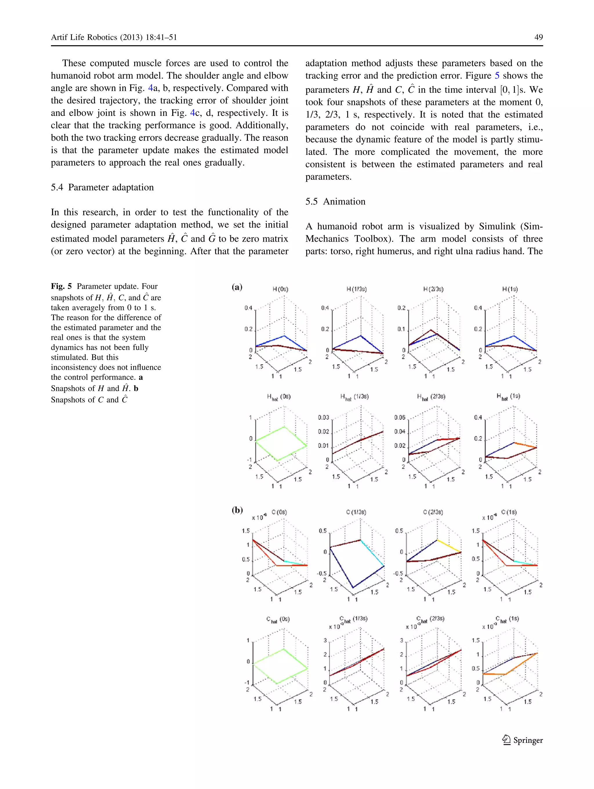
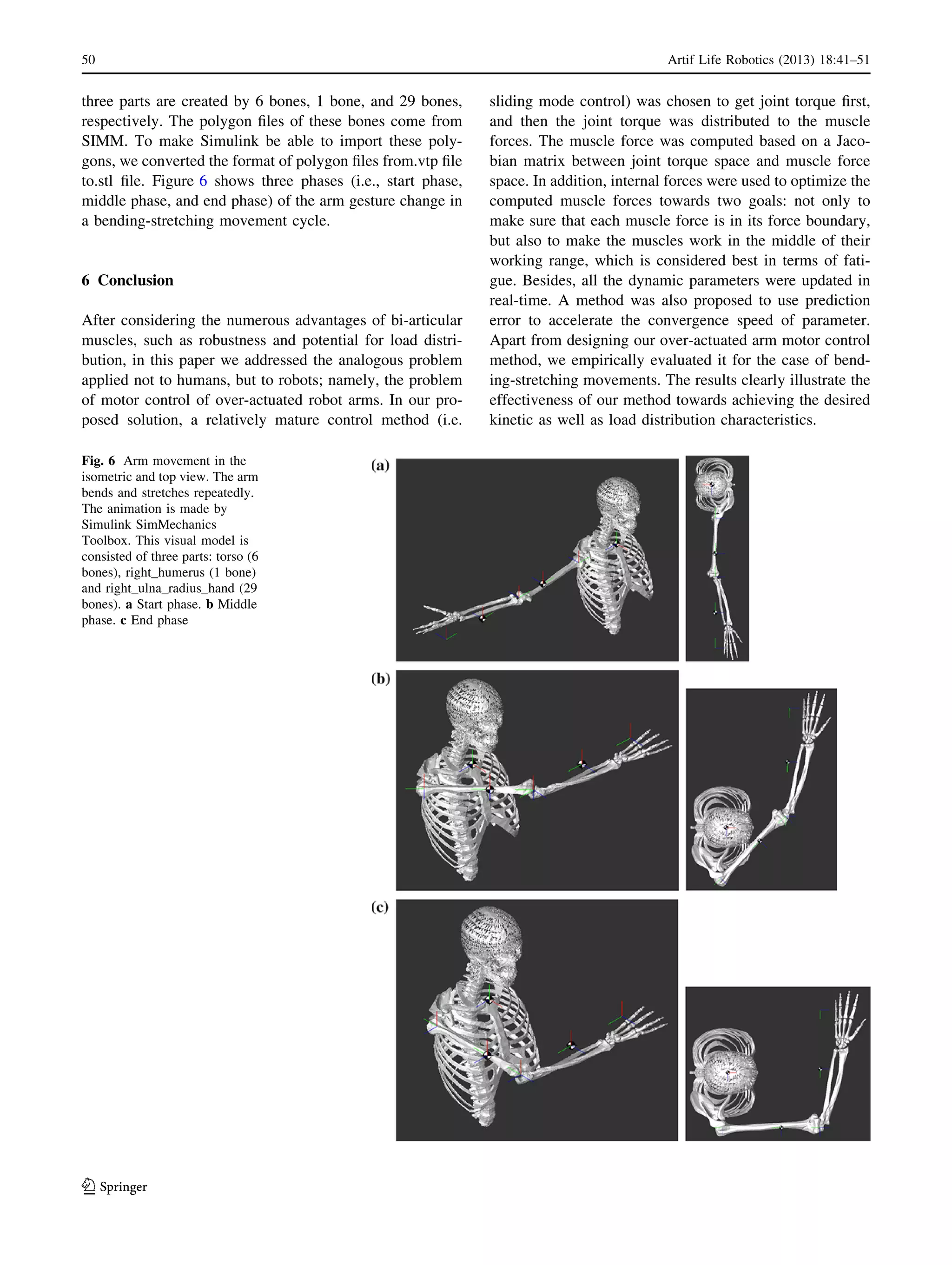
This document summarizes a research paper about developing an adaptive control method for a humanoid robot arm with bi-articular and mono-articular muscle mechanisms. The researchers used sliding mode control to first determine joint torques, then distributed those torques to muscle forces using a Jacobian matrix. Internal forces were also used to optimize muscle forces so they remained within limits and worked in the middle of their range to reduce fatigue. Dynamic parameters were updated in real-time using a novel method of prediction error to accelerate parameter convergence. The results showed the effectiveness of the proposed method in achieving desired motion and load distribution characteristics.
![ORIGINAL ARTICLE
Muscle force distribution for adaptive control of a humanoid
robot arm with redundant bi-articular and mono-articular muscle
mechanism
Haiwei Dong • Nikolaos Mavridis
Received: 7 January 2013 / Accepted: 14 May 2013 / Published online: 30 May 2013
Ó ISAROB 2013
Abstract Robot arms driven by bi-articular and mono-
articular muscles have numerous advantages. If one muscle
is broken, the functionality of the arm is not influenced. In
addition, each joint torque is distributed to numerous
muscles, and thus the load of each muscle can be relatively
small. This paper addresses the problem of muscle control
for this kind of robot arm. A relatively mature control
method (i.e. sliding mode control) was chosen to get joint
torque first and then the joint torque was distributed to
muscle forces. The muscle force was computed based on a
Jacobian matrix between joint torque space and muscle
force space. In addition, internal forces were used to
optimize the computed muscle forces in the following
manner: not only to make sure that each muscle force is in
its force boundary, but also to make the muscles work in
the middle of their working range, which is considered best
in terms of fatigue. Besides, all the dynamic parameters
were updated in real-time. Compared with previous work, a
novel method was proposed to use prediction error to
accelerate the convergence speed of parameter. We
empirically evaluated our method for the case of bending-
stretching movements. The results clearly illustrate the
effectiveness of our method towards achieving the desired
kinetic as well as load distribution characteristics.
Keywords Muscle cooperation Á Redundancy Á
Internal force Á Parameter adaptation
1 Introduction
1.1 Background
Traditional robot arms are driven by motors. Each motor
drives a specific joint, corresponding to an independent
degree of freedom (DOF). There are two main problems in
this approach. First, if one motor is broken, the DOF cor-
responding to this motor will be lost. Second, the motor
near the base link always needs more power, leading to a
requirement for very heavy motors near the base. But let us
compare this to the human motor system: as there are many
muscles driving one joint, the total joint torque is distrib-
uted to every muscle. Thus, each muscle only carries a
relatively small load. Furthermore, if one muscle is broken,
the function of rotation for the corresponding joint does not
change. Thus, recently such driving systems for robots
inspired by muscles have started to be explored, creating a
new research direction. For example, there are a number of
papers focusing on bionic arms [1–4]. In our work, we
propose a muscle control method for humanoid robot arm
driven by bi-articular muscles. Here, the control method is
designed to be adaptive, i.e. robust to perturbations and
disturbances from environment. In addition, the muscle
forces have to satisfy the boundary force limit. Last, but
quite importantly, the method has to be efficient enough for
practical application.
To get insight into this muscle control problem, we can
consider it through viewpoints arising from two research
fields: human motor control and robotics. In human motor
control, the human body is usually considered as a multi-
link rigid body with numerous joints. By adding muscles
and tensors, the human body moves according to control
signals arising from the neural system. Such a kind of
system is usually termed a neural-skeleton muscle system
H. Dong (&) Á N. Mavridis
New York University AD, P.O. Box 129188, Abu Dhabi, UAE
e-mail: haiwei.dong@nyu.edu
N. Mavridis
e-mail: nikolaos.mavridis@nyu.edu
123
Artif Life Robotics (2013) 18:41–51
DOI 10.1007/s10015-013-0097-x](https://image.slidesharecdn.com/2013artificiallifeandrobotics-140523201753-phpapp02/75/Muscle-force-distribution-for-adaptive-control-of-a-humanoid-robot-arm-with-redundant-bi-articular-and-mono-articular-muscle-mechanism-1-2048.jpg)
![[5, 6] and the muscle control is described as human motor
control [7]. On the other hand, in robotics, there is also a
related research field focusing on controlling multi-link
rigid bodies [8–10].
In our research, we face two problems: redundancy and
adaptivity. For redundancy, there exist two types of
redundancies here. Type I Redundancy is between end
effector position and joints. Taking the robot arm as an
example, the number of degrees of freedom (DOF) of the
end effector position is 3, i.e., the end effector can move in
3D space. Nevertheless, the number of joints in the arm can
be more than 3, indicating the fact that for the same end
effector position, there exist many limb joint configura-
tions. The other type of redundancy, Type II Redundancy,
is between joint torque and muscle force. In the human
motor system, there are many more muscles as compared
to the minimum number required to generate the full range
of required movement [11, 12]. Towards generating a
certain desired joint torque, there is a lot of flexibility in
distributing load among the cooperating muscles. For
example, if we ask a subject to keep a certain gesture, when
the subject is under nervous status, the muscles are tense.
Both agonist muscles and antagonist muscles output large
force. At this time, the body’s impedance status is in a self-
protection mode, and the damping and viscosity coeffi-
cients are correspondingly large [13, 14]. Conversely,
when the subject is under relaxation status, the muscle
force, damping and viscosity coefficients are small. The
above two extreme statuses correspond to the same zero
joint torque with different muscle force distributions.
Ability for adaptation is also a very important issue,
especially for humanoid robots. As humanoid robots are
usually tailored towards significant human–robot interac-
tion, often their working environment is mainly a human
environment, which is very complex and always accom-
panied with various kinds of uncertainties. Furthermore,
even if we do not consider the environmental uncertainty,
and we focus on the robot itself, we still often have robot
model errors. Thus, in order to be able to create humanoids
that perform adequately under such conditions, it is nec-
essary to propose methods that have the ability to perform
real-time adaptation, for counteracting such uncertainties.
1.2 Related work
Let us start by discussing relevant work in human–robot
control, and then moving over to relevant work in robotics.
In human motor control, two of the main research direc-
tions are those focusing towards redundancy solutions and
ability for adaptation. Let us start with the first: redundancy
solution. The basic method utilized is nonlinear optimiza-
tion [15–18]. There have been many successful applica-
tions. Hogan proposed a voluntary movement principle
using dynamic optimization which minimizes the rate of
acceleration change of the limb [19]. Anderson et al. [15]
used dynamic optimization of minimum metabolic energy
expenditure to solve the motion control of walking. Manal
et al. [11] designed a nonlinear optimal controller to
develop a real-time EMG-driven virtual arm. Neptune [16]
evaluated different multivariate optimization methods in
pedaling.
The optimization method in human motor control
includes two different kinds of methods. One is forward
dynamics method which uses muscle excitations as the
inputs to calculating the corresponding body motions [12,
20]. It is a novel research in forward dynamics that
Anderson et al. [21] uses a parallel computer to calculate
the derivatives of the cost function and the constraints with
each control variable. The other is inverse dynamics
method [18]. Noninvasive measurement of body motions
(position, velocity, and acceleration of each segment) and
external forces are used as inputs to calculate muscle for-
ces. Two commercial software packages are famous based
on these two methods: AnyBody Modeling System as
inverse dynamics method [22] and OpenSim as forward
dynamics method [23].
As mentioned above, a second main research direction
focuses on adaptation ability. Although adaptation ability
based on bio-feedback has not been fully understood in
human motor control, right now the basic comprehension is
a combination control scheme of feed-forward control and
feedback control [24]. The feed-forward control corre-
sponds to the inverse dynamics [25–27]. Specifically, the
inverse dynamics are learnt (i.e., estimated) by nervous
system. Then, the feedback control uses this inverse
dynamics to provide a basic control efficiently. The feed-
back control deals with environment disturbance, load
change, and learning error of inverse dynamics, etc. It is
usually considered as a Visual Servo Feedback System
[28].
Now let us move from human motor control to
robotics. In robotics, modeling and control of multi-link
rigid body (especially manipulator control) have been
studied for years [10, 29–31]. Here, the redundancy
problem is usually considered from the viewpoint of
dynamic control [1, 32]. For Type I Redundancy problem,
considering different optimization criterion or restricted
conditions, many methods have been proposed. Yoshika-
wa [29] proposed a manipulability measure, by mini-
mizing which the arm is kept away from singularities.
Maciejewski et al. [30] used null-space vector to aid
obstacle avoidance. For Type II Redundancy problem,
there have been researches on building bionic robots to
mimic human’s movement system. Klug et al. [2]
developed a 3 DOF bionic robot arm which is controlled
by a PD controller with feed-forward compensation. The
42 Artif Life Robotics (2013) 18:41–51
123](https://image.slidesharecdn.com/2013artificiallifeandrobotics-140523201753-phpapp02/75/Muscle-force-distribution-for-adaptive-control-of-a-humanoid-robot-arm-with-redundant-bi-articular-and-mono-articular-muscle-mechanism-2-2048.jpg)
![trajectory of the arm is optimized and adjusted for a time
and energy-optimal motion [33]. Potkonjak et al. [3] built
a humanoid robot with antagonistic drives whose con-
troller is designed by H1 loop shaping. Tahara [4] pro-
posed a simple sensor-motor control scheme as internal
force and simulated the overall stability.
The initial research on adaptation ability in robotics
comes from online system identification. The objective is
to estimate system structure and parameters in real-time.
Here, the system is considered as a black box or gray box.
By stimulating the system and creating relation between
the inputs and outputs, the parameters of the system can be
adjusted online [34]. Based on this identification idea,
many adaptive methods came out, such as robust control
[35], adaptive feedback control [36], neurofuzzy adaptive
control [37], etc. However, the adaptation ability problem
has not been considered in arm control by bi-articular
muscles.
1.3 Our solution
In this paper, we took into account the previous research in
human motor control and robotics. One of our initial
observations was that the optimization-series methods are
difficult to use in practical applications because of their
relative inefficiency and difficulty in dealing with. It is also
difficult to directly propose a muscle control method for the
robot arm as it is hard to decouple the two redundancies.
Therefore, we use a relatively mature control method (i.e.
sliding mode control) to get joint torque first and then
distribute the joint torque to muscle forces. The muscle
force was computed based on a Jacobian matrix between
joint torque space and muscle force space. In addition,
internal forces were used to optimize the computed muscle
forces in the following manner: not only to make sure that
each muscle force is in its force boundary, but also to make
the muscles work in the middle of their working range,
which is considered best in terms of fatigue. Besides, all
the dynamic parameters were updated in real-time. A novel
method was proposed to use prediction error to accelerate
the convergence speed of parameter. We empirically
evaluated our method for the case of bending-stretching
movements. The results clearly illustrate the effectiveness
of our method towards achieving the desired kinetic as well
as load distribution characteristics.
2 Modeling arm with muscles
2.1 Arm model
We built a 2-dimensional model of the arm in the hori-
zontal plane based on the upper limb structure of a digital
human. The model includes six muscles (shown as 1–6)
and two degrees of freedom (shoulder flexion–extension
and elbow flexion–extension). The range of shoulder angle
is from -20 to 100°, and the range of the elbow is from 0
to 170°. Four of the muscles are mono-articular, and two
are bi-articular where 1 and 2 cross the shoulder joint; 3
and 4 cross the elbow joint; 5 and 6 cross both joints
(Fig. 1).
Considering the arm (including upper arm and lower
arm) as a planar, two-link, articulated rigid object, the
position of hand can be derived by a 2-vector q of two
angles. The input is a 6-vector Fm of muscle forces.
The dynamics of the rigid object is strongly nonlinear.
Using the Lagrangian equations in classical dynamics,
we get the dynamic equations of the ideal upper limb
model
H11 tð Þ H12 tð Þ
H21 tð Þ H22 tð Þ
!
€q1
€q2
!
þ
C11 tð Þ C12 tð Þ
C21 tð Þ C22 tð Þ
!
_q1
_q2
!
þ
G1 tð Þ
G2 tð Þ
!
¼
s1 tð Þ
s2 tð Þ
!
ð1Þ
or abbreviated as
H tð Þ€q þ C tð Þ _q þ G tð Þ ¼ s ð2Þ
with q ¼ q1 q2½ ŠT
¼ h1 h2½ ŠT
being the two joint
angles. s ¼ s1 s2½ ŠT
¼ f Fmð Þ is a function of muscle
force Fm
Fm ¼ Fm;1 Fm;2 Fm;3 Fm;4 Fm;5 Fm;6½ ŠT
ð3Þ
H q; tð Þ is inertia matrix containing information with
regard to the instantaneous mass distribution. C q; _q; tð Þ is
centripetal and coriolis torques representing the moments
Fig. 1 Humanoid robot arm model. The arm has two degrees of
freedom and it can rotate around the shoulder angle and elbow angle
in the anterior plane
Artif Life Robotics (2013) 18:41–51 43
123](https://image.slidesharecdn.com/2013artificiallifeandrobotics-140523201753-phpapp02/75/Muscle-force-distribution-for-adaptive-control-of-a-humanoid-robot-arm-with-redundant-bi-articular-and-mono-articular-muscle-mechanism-3-2048.jpg)
![of centrifugal forces. G q; tð Þ is gravitational torques
changing with the posture configuration of the arm.
H11 ¼ J1 þ J2 þ m2d2
1 þ 2m2d1c2 cos q2ð Þ
H12 ¼ H21 ¼ J2 þ m2d1c2 cos q2ð Þ
H22 ¼ J2
C11 ¼ À2m2d1c2 sin q2ð Þ _q2
C12 ¼ Àm2d1c2 sin q2ð Þ _q2
C21 ¼ m2d1c2 sin q2ð Þ _q1
C22 ¼ 0
G1 ¼ g m1c1 þ m2d1ð Þ cos q1ð Þ þ gm2c2 cos q1 þ q2ð Þ
G2 ¼ gm2c2 cos q1 þ q2ð Þ; ð4Þ
where g is the acceleration of gravity. ci is the distance
from the center of a joint i to the center of the gravity point
of link i: di is the length of link i. Ji ¼ mid2
i þ Ii where Ii is
the moment of inertia about axis through the center of mass
of link i.
2.2 Model with estimated parameters
In our research, we consider the arm model in Eq. (1) is
influenced by disturbances and perturbations from the
environment. Hence, we used an estimated arm model to
control, which is written as
^H11 tð Þ ^H12 tð Þ
^H21 tð Þ ^H22 tð Þ
" #
€q1
€q2
!
þ
^C11 tð Þ ^C12 tð Þ
^C21 tð Þ ^C22 tð Þ
" #
_q1
_q2
!
þ
^G1 tð Þ
^G2 tð Þ
" #
¼
^s1 tð Þ
^s2 tð Þ
!
ð5Þ
or abbreviated as
^H tð Þ€q þ ^C tð Þ _q þ ^G tð Þ ¼ ^s; ð6Þ
where ^Á means estimated value of Áð Þ. The connection part
between ideal model (Eq. 1) and estimated model (Eq. 5)
is that we choose s ¼ ^s. Below, we use estimated model (5)
to generate torque for real system for control. In addition,
the parameter adaptation updates the estimated parameters
^H, ^C and ^G in real time.
2.3 Dynamic parameters definition
For the convenience of following derivation, we define the
actual and estimated arm parameter vector
P ¼ PT
H PT
C PT
G
 ÃT
; ^P ¼ ^PT
H
^PT
C
^PT
G
 ÃT
; ð7Þ
where
PH ¼
H11
H12
H21
H22
2
6
6
6
4
3
7
7
7
5
; PC ¼
C11
C12
C21
C22
2
6
6
6
4
3
7
7
7
5
; PG ¼
G1
G2
!
;
^PH ¼
^H11
^H12
^H21
^H22
2
6
6
6
4
3
7
7
7
5
; ^PC ¼
^C11
^C12
^C21
^C22
2
6
6
6
4
3
7
7
7
5
; ^PG ¼
^G1
^G2
" #
ð8Þ
then the estimation error vector can be defined as
~P ¼ ^P À P ¼ ~PT
H
~PT
C
~PT
G
 ÃT
: ð9Þ
3 Joint torque computation
3.1 Torque control method
Sliding mode control is used to control the posture of the
arm [36]. A 2-vector qd is the desired states. Define a
sliding mode term s as
s ¼ _~q þ K~q ¼ ð _q À _qdÞ þ Kðq À qdÞ ð10Þ
where K is a positive diagonal matrix. Defining the
reference velocity _qr and reference acceleration €qr as
_qr ¼ _q À s
€qr ¼ €q À _s
ð11Þ
then we choose the control method as
s ¼ ^HðqÞ€qr þ ^Cðq; _qÞ _qr þ ^G À KsgnðsÞ; ð12Þ
where K is convergence parameter which is a diagonal
matrix. The proof of sliding mode control is in [38].
3.2 Parameter adaptation method
To accelerate the parameter update speed, we use two error
sources to update estimated parameters. The first source is
tracking error. We chose the parameter adaptation method
based on tracking error as
_^Ptra ¼ ÀCÀ1
s1 €qT
r s2 €qT
r s1 _qT
r s2 _qT
r s1 s2
 ÃT
; ð13Þ
where C is adaptation parameter which is a diagonal
matrix. The derivation of this parameter adaptation method
is based on the sliding mode control method, which is
proved in [39].
On the other side, the dynamic equation (Eq. 1) can be
written in the form
s tð Þ ¼
€q1 0 €q1 0 _q1 0 _q1 0 1 0
0 €q2 0 €q2 0 _q2 0 _q2 0 1
! PH
PC
PG
2
4
3
5:
ð14Þ
44 Artif Life Robotics (2013) 18:41–51
123](https://image.slidesharecdn.com/2013artificiallifeandrobotics-140523201753-phpapp02/75/Muscle-force-distribution-for-adaptive-control-of-a-humanoid-robot-arm-with-redundant-bi-articular-and-mono-articular-muscle-mechanism-4-2048.jpg)
![After simplification, we finally get
l1 ¼ a2
11 þ a2
12 þ 2a11a12 cos h1ð Þ
À Á1=2
l2 ¼ a2
21 þ a2
22 À 2a21a22 cos h1ð Þ
À Á1=2
l3 ¼ a2
31 þ a2
32 þ 2a31a32 cos h2ð Þ
À Á1=2
l4 ¼ a2
41 þ a2
42 À 2a41a42 cos h2ð Þ
À Á1=2
l5 ¼ a51 þ a01ð Þ2
þ a52 þ a02ð Þ2
þ2 a51 þ a01ð Þ a52 þ a02ð Þ
 cos h1 þ h2ð ÞÞ1=2
l6 ¼ a01 À a61ð Þ2
þ a02 À a62ð Þ2
þ2 a01 À a61ð Þ a02 À a62ð Þ
 cos h1 þ h2ð ÞÞ1=2
ð28Þ
Assuming the kinematics between the length of muscle
and the angle of joint is given as follows
L ¼ Q Hð Þ ð29Þ
where
L ¼ l1 l2 l3 l4 l5 l6½ ŠT
H ¼ h1 h2½ ŠT ð30Þ
then the derivative of Eq. (29) is
_L ¼ Jm
_H ð31Þ
where Jm is a Jacobian matrix between the joint space and
the muscle space. It has a format as
Jm ¼
Jm;1;1 Jm;1;2
Jm;2;1 Jm;2;2
Jm;3;1 Jm;3;2
Jm;4;1 Jm;4;2
Jm;5;1 Jm;5;2
Jm;6;1 Jm;6;2
2
6
6
6
6
6
6
4
3
7
7
7
7
7
7
5
; ð32Þ
where
Jm;1;1 ¼
Àa11a12 sin h1ð Þ
ffiffiffiffiffiffiffiffiffiffiffiffiffiffiffiffiffiffiffiffiffiffiffiffiffiffiffiffiffiffiffiffiffiffiffiffiffiffiffiffiffiffiffiffiffiffiffiffiffiffiffiffiffiffi
a2
11 þ 2 cos h1ð Þa11a12 þ a2
12
p
Jm;2;1 ¼
Àa21a22 sin h1ð Þ
ffiffiffiffiffiffiffiffiffiffiffiffiffiffiffiffiffiffiffiffiffiffiffiffiffiffiffiffiffiffiffiffiffiffiffiffiffiffiffiffiffiffiffiffiffiffiffiffiffiffiffiffiffiffi
a2
21 þ 2 cos h1ð Þa21a22 þ a2
22
p
Jm;3;2 ¼
Àa31a32 sin h2ð Þ
ffiffiffiffiffiffiffiffiffiffiffiffiffiffiffiffiffiffiffiffiffiffiffiffiffiffiffiffiffiffiffiffiffiffiffiffiffiffiffiffiffiffiffiffiffiffiffiffiffiffiffiffiffiffi
a2
31 þ 2 cos h2ð Þa31a32 þ a2
32
p
Jm;4;2 ¼
a41a42 sin h2ð Þ
ffiffiffiffiffiffiffiffiffiffiffiffiffiffiffiffiffiffiffiffiffiffiffiffiffiffiffiffiffiffiffiffiffiffiffiffiffiffiffiffiffiffiffiffiffiffiffiffiffiffiffiffiffiffi
a2
41 þ 2 cos h2ð Þa41a42 þ a2
42
p
Jm;1;2 ¼ Jm;2;2 ¼ Jm;3;1 ¼ Jm;4;1 ¼ 0
ð33Þ
Jm;5;1, Jm;5;2, Jm;6;1 and Jm;6;2 are long equations and we
do not provide them here. The derivation of the above
Jacobian matrix can be done by Matlab Symbolic Toolbox.
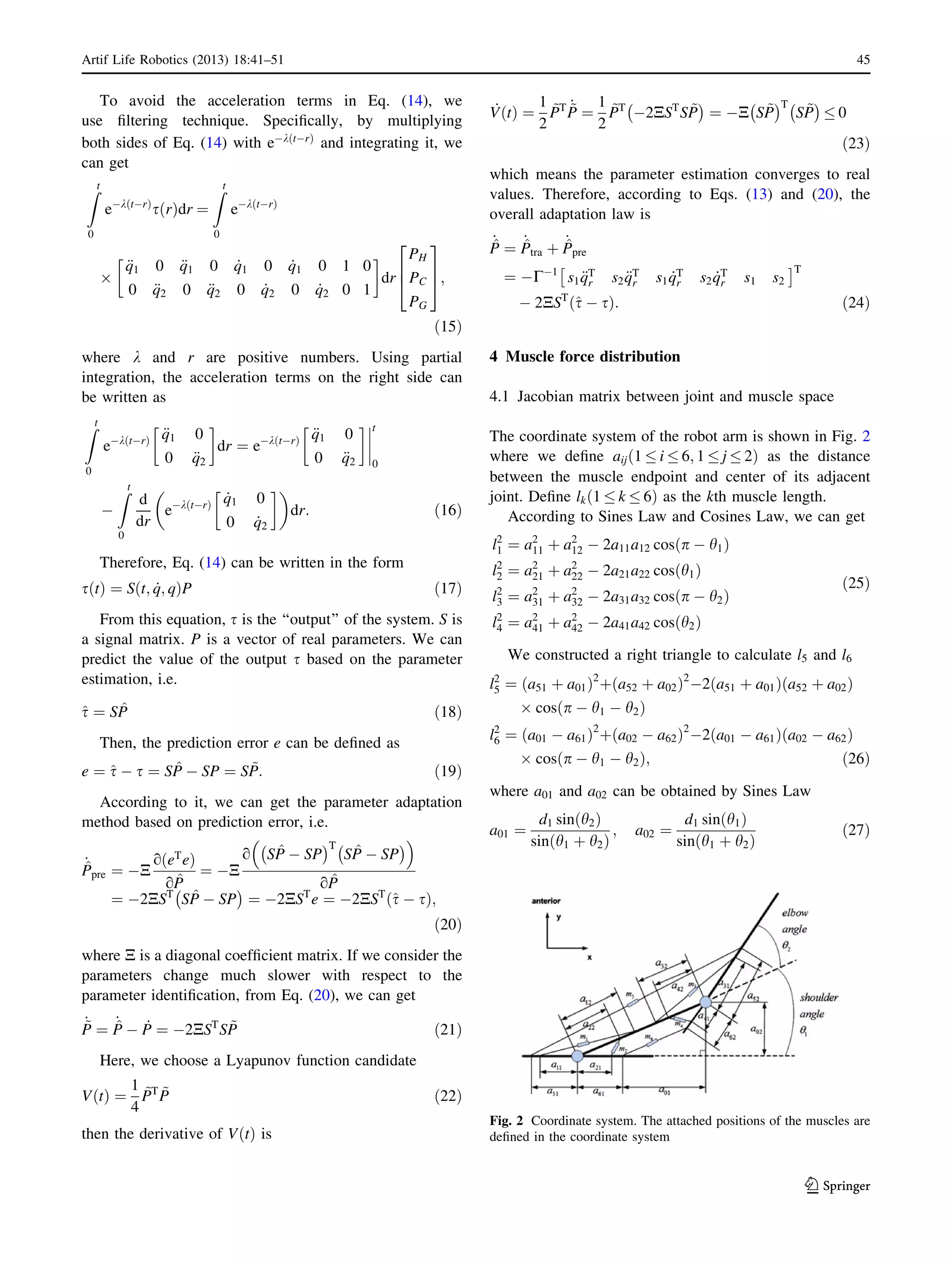
4.2 Muscle force distribution
The relationship between muscle forces and joint torques
can be derived by the principle of virtual work as
s ¼ f Fmð Þ ¼ JT
mFm: ð34Þ
Hence, the inverse relation between the joint torques and
the muscle forces can be expressed as
sinv ¼ fÀ1
sð Þ ¼ JT
m
À Áþ
s ð35Þ
where
JT
m
À Áþ
¼ Jm JT
mJm
À ÁÀ1
ð36Þ
is pseudo-inverse matrix of JT
m. The above muscle force
distribution solution satisfies
min Fmk k
s:t: JT
mFm ¼ s
ð37Þ
which means the pseudoinverse is an optimization solution
to obtain minimums muscle distribution force. However,
the above solution does not consider physical constraints,
such as the maximum output force of muscle is limited,
muscles can only contract, etc. To involve these
constraints, we define Fin as a voluntary vector having
the same dimension with Fm which expresses the internal
forces generated by redundant muscles. Then, we can
define the internal force in Fm space, i.e.
g Finð Þ ¼ I À JT
m
À Áþ
JT
m
Fin ð38Þ
where I is an identity matrix having the same dimension
with muscle space. According to Moore–Penrose pseudo-
inverse, g Finð Þ is orthogonal with the pseudo-inverse
solution. Thus, we can choose any vector as Fin. Below, we
give a gradient direction for Fin to make Fm satisfy
boundary constraints.
Here, we assume that each muscle force is limited in the
interval from Fm;i;min to Fm;i;max for 1 i 6. Our objective
is to choose a gradient direction to make each element of
Fm;i 1 i 6ð Þ equal or greater than Fm;i;min, and equal or
Table 1 Anthropological parameter values
Segment Upper arm Lower arm
Length (m) 0.282 0.269
Mass (kg) 1.980 1.180
MCS Pos (m) 0.163 0.123
I11 (kg m2
) 0.013 0.007
I22 (kg m2
) 0.004 0.001
I33 (kg m2
) 0.011 0.006
The parameter setting of the arm is based on a real human data [40]
MCS Pos position of the mass center
46 Artif Life Robotics (2013) 18:41–51
123](https://image.slidesharecdn.com/2013artificiallifeandrobotics-140523201753-phpapp02/75/Muscle-force-distribution-for-adaptive-control-of-a-humanoid-robot-arm-with-redundant-bi-articular-and-mono-articular-muscle-mechanism-6-2048.jpg)
![less than Fm;i;max. Considering the muscle fatigue, one
reasonable way is to make each output force of the muscles
to be around at the middle magnitude between Fm;i;min and
Fm;i;max. The physical meaning of this method is to dis-
tribute load to all the muscles in their proper load interval,
so that they can continue working for a longer time. Based
on these considerations, we choose a function h as
h Fmð Þ ¼
X6
j¼1
sinv;i À Fm;i;mid
Fm;i;mid À Fm;i;max
2
ð39Þ
where
0 Fm;i;min sinv;i Fm;i;max
Fm;i;mid ¼
Fm;i;min þ Fm;i;max
2
i ¼ 1; 2; . . .6 ð40Þ
then we chose Fin as the gradient of the function h, i.e.
Fin ¼ Kin
oh sinvð Þ
osinv
¼ Kinrh ¼ Kin
2 Á
sinv;1ÀFm;1;mid
Fm;1;midÀFm;1;max
2 Á
sinv;2ÀFm;2;mid
Fm;2;midÀFm;2;max
2 Á
sinv;3ÀFm;3;mid
Fm;3;midÀFm;3;max
2 Á
sinv;4ÀFm;4;mid
Fm;4;midÀFm;4;max
2 Á
sinv;5ÀFm;5;mid
Fm;5;midÀFm;5;max
2 Á
sinv;6ÀFm;6;mid
Fm;6;midÀFm;6;max
2
6
6
6
6
6
6
6
6
6
6
4
3
7
7
7
7
7
7
7
7
7
7
5
ð41Þ
where Kin is a scalar matrix. It is very easy to prove that the
direction of Fin points to Fm;i;mid. According to the
computation in Eqs. (35) and (41), the muscle force is
calculated as
Fm ¼ sinv þ g Finð Þ ð42Þ
The procedures to compute muscle force are concluded
as the following algorithm.
5 Bending-streching movement simulation
The performance of the proposed muscle force computa-
tion method was tested by simulation. The desired
movement is bending the upper arm and lower arm from
0 rad to p=2 rad and then stretching them back to 0 rad.
The total simulation time was 10 s.
5.1 Arm model parameter setting
The parameters of the robot arm are based on the real data
of a human upper limb. The setting of length, mass, mass
center position and inertia coefficients is shown in Table 1.
The anthropological data come from [40]. Without loss of
generality, the muscle configuration coefficients (in Eq. 28)
are set as aij ¼ 0:1m 1 i 6; 1 j 2ð Þ.
5.2 Computational coefficient setting
There are three groups of parameters need to set, including
the parameters for sliding mode control, the parameters for
parameter adaptation, and the parameters for muscle force
computation. These parameters are set as follows.
In this research, the control parameters are set (Eq. 12)
as
K ¼ 20 Á Diag 1 1½ Šð Þ ð43Þ
the adaptation parameters (Eq. 24) are set as
CÀ1
¼ 0:0015 Á Diag 1 1 1 1 1 1 1 1 1 1½ Šð Þ
2N ¼ 0:001 Á Diag 1 1 1 1 1 1 1 1 1 1½ Šð Þ
ð44Þ
and the muscle force computation parameters (Eq. 41) are
set as
Kin ¼ 200 Á Diag 1 3 1 1 1 2½ Šð Þ ð45Þ
Fm;i;min ¼ 0; Fm;i;max ¼ 1000 1 i 6ð Þ; ð46Þ
where Diag Áð Þ is a diagonal matrix with diagonal elements
being as Áð Þ.
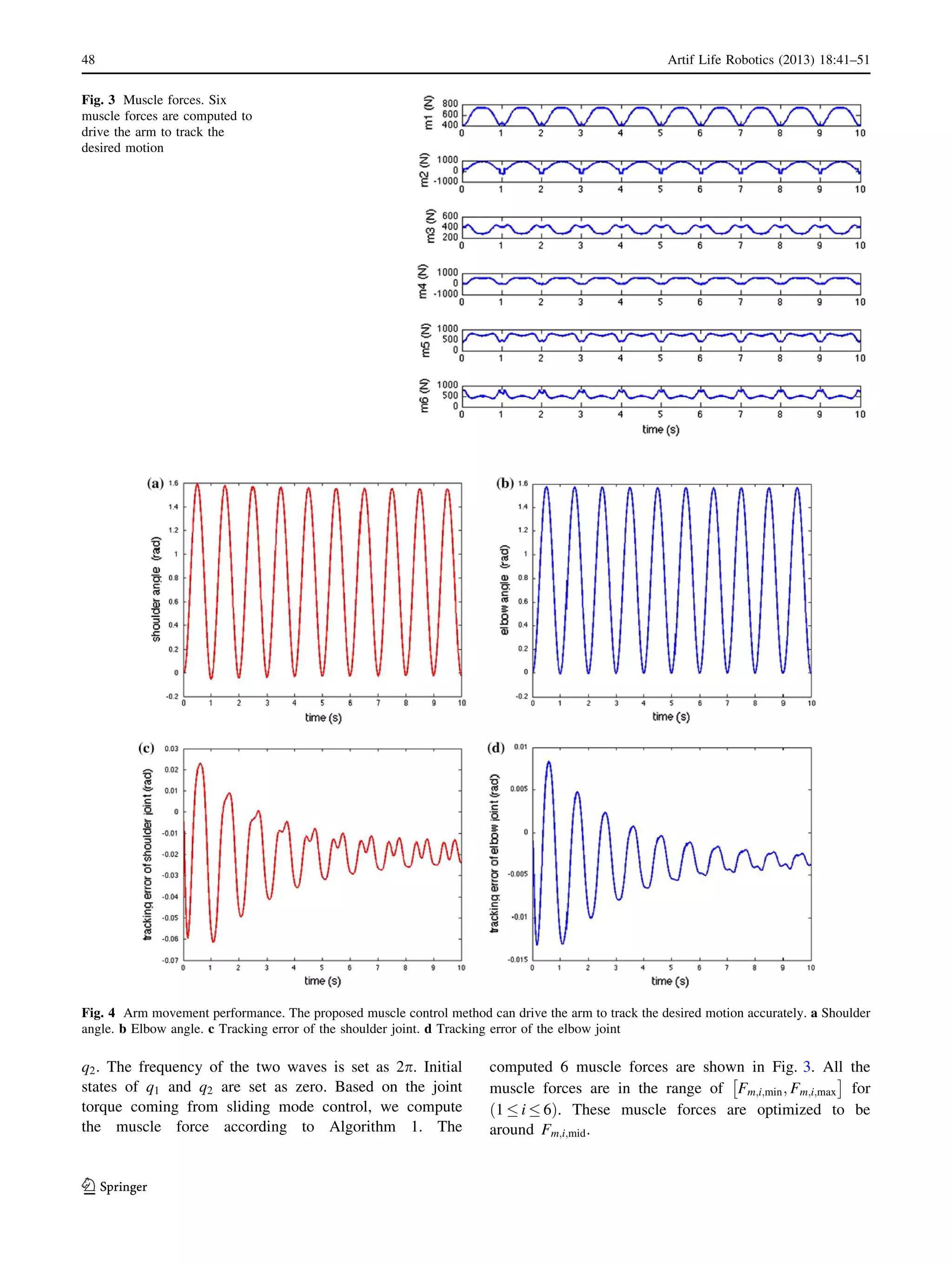
5.3 Control performance
According to the bending-stretching movement, two
sinusoidal waves are set as reference signals for q1 and
Algorithm 1 Muscle force distribution
Step 1 Computing Jacobian matrix (Eq. (32)) according to Eq. (33).
Step 2 Computing pseudoinverse matrix according to Eq. (36).
Step 3 Computing according to Eq. (35).
Step 4 Computing internal force according to Eq. (41). Here, comes
from the result in Step 3.
Step 5 Computing according to Eq. (38).
Step 6 Computing muscle force by Eq. (42) where comes from Step 3 and
comes from Step 5.
Jm
Fin
Fin
τinv
τinv
τinv,i
g
Jm( (
( (
Fing( (
(1 ≤ i ≤ 6)
T +
Artif Life Robotics (2013) 18:41–51 47
123](https://image.slidesharecdn.com/2013artificiallifeandrobotics-140523201753-phpapp02/75/Muscle-force-distribution-for-adaptive-control-of-a-humanoid-robot-arm-with-redundant-bi-articular-and-mono-articular-muscle-mechanism-7-2048.jpg)


![ICNR2016_Knuth[1384]](https://cdn.slidesharecdn.com/ss_thumbnails/6c67b0f5-4fc6-46ef-8f35-499ef5c55f5a-170203174039-thumbnail.jpg?width=640&height=640&fit=bounds)


