This document describes the development and testing of an EMG-driven musculoskeletal model to estimate muscle forces and knee joint moments in vivo. The model uses EMG and joint kinematic data as inputs to estimate individual muscle forces and resulting knee joint moments. The model was calibrated for six individuals by adjusting physiological parameters to match net flexion/extension muscle moments measured through inverse dynamics. Once calibrated, the model predicted knee joint moments across over 200 dynamic tasks with high accuracy (average R2 of 0.91), demonstrating the model's ability to estimate muscle forces and joint moments over a wide range of dynamic conditions.

1. Journal of Biomechanics 36 (2003) 765–776
An EMG-driven musculoskeletal model to estimate muscle forces and
knee joint moments in vivo
David G. Lloyd*, Thor F. Besier
School of Human Movement & Exercise Science, University of Western Australia, Perth, 35 Stirling Highway, Crawley, WA 6009, Australia
Accepted 19 December 2002
Abstract
This paper examined if an electromyography (EMG) driven musculoskeletal model of the human knee could be used to predict
knee moments, calculated using inverse dynamics, across a varied range of dynamic contractile conditions. Muscle–tendon lengths
and moment arms of 13 muscles crossing the knee joint were determined from joint kinematics using a three-dimensional anatomical
model of the lower limb. Muscle activation was determined using a second-order discrete non-linear model using rectified and low-
pass filtered EMG as input. A modified Hill-type muscle model was used to calculate individual muscle forces using activation and
muscle tendon lengths as inputs. The model was calibrated to six individuals by altering a set of physiologically based parameters
using mathematical optimisation to match the net flexion/extension (FE) muscle moment with those measured by inverse dynamics.
The model was calibrated for each subject using 5 different tasks, including passive and active FE in an isokinetic dynamometer,
running, and cutting manoeuvres recorded using three-dimensional motion analysis. Once calibrated, the model was used to predict
the FE moments, estimated via inverse dynamics, from over 200 isokinetic dynamometer, running and sidestepping tasks. The
inverse dynamics joint moments were predicted with an average R2
of 0.91 and mean residual error of B12 Nm. A re-calibration of
only the EMG-to-activation parameters revealed FE moments prediction across weeks of similar accuracy. Changing the muscle
model to one that is more physiologically correct produced better predictions. The modelling method presented represents a good
way to estimate in vivo muscle forces during movement tasks.
r 2003 Elsevier Science Ltd. All rights reserved.
Keywords: EMG-driven model; Musculoskeletal model; Knee biomechanics
1. Introduction
Measuring the forces applied to a joint and estimating
how these forces are partitioned to surrounding muscles,
ligaments, and articular surfaces is fundamental to
understanding joint function, injury, and disease.
Inverse dynamics can be used to estimate the external
load applied to a joint, however, the contribution from
muscles to support or generate this load is far more
difficult to determine given the indeterminate nature of
the joint. One solution to this problem is to estimate
muscle forces based on an objective function within an
optimisation routine, for example, minimising muscle
stress. By default, the use of an objective function
cannot account individual muscle activation patterns.
Another solution uses electromyography (EMG) in
conjunction with an appropriate anatomical and muscle
model to estimate the forces produced in each muscle
(e.g. Lloyd and Buchanan, 1996; McGill, 1992). Since
‘EMG-driven’ models rely on measured muscle activity
to estimate muscle force, these models implicitly account
for a subject’s individual activation patterns without the
need to satisfy any constraints imposed by an objective
function. This is important if we wish to investigate
tissue loading throughout a wide range of tasks and
contractile conditions, as the activation of muscle
depends on the control task and can be quite different
for the same joint angle and joint torque (Tax et al.,
1990; Buchanan and Lloyd, 1995). Indeed, in isometric
tasks Lloyd and Buchanan (2001) showed quite different
activation patterns between subjects to generate the same
relative knee moments in flexion/extension and varus/
valgus directions, resulting in quite different amounts of
support provided by the muscles and ligaments.
*Corresponding author. Tel.: +61-9-380-3919; fax: +61-9-380-
1039.
E-mail address: dlloyd@cyllene.uwa.edu.au (D.G. Lloyd).
0021-9290/03/$ - see front matter r 2003 Elsevier Science Ltd. All rights reserved.
doi:10.1016/S0021-9290(03)00010-1

2. EMG-driven models have been developed to estimate
muscle forces for the lower back (McGill and Norman,
1986; McGill, 1992; Granata and Marras, 1993; Thelen
et al., 1994; Nussbaum and Chaffin, 1998), elbow
(Soechting and Flanders, 1997; Buchanan et al., 1998),
shoulder (Laursen et al., 1998), knee (White and Winter,
1993; Lloyd and Buchanan, 1996; Piazza and Delp,
1996), and ankle (Hof and van den Berg, 1981a, b). As
direct measures of muscle force in vivo are difficult,
EMG-driven models are typically validated to external
joint moments measured using an inverse dynamics
approach. The ability of EMG-driven models to predict
joint moments during a wide range of activities has
proven difficult in the past, and several methods have
been devised to satisfy this moment constraint. One such
method involves using an error term or ‘gain’ to ensure
the predicted moments from a model match the
externally measured moments for each task (e.g. McGill,
1992). An alternate method involves using a non-linear
least squares optimisation procedure to alter specific
parameters within the model to ensure that the moment
constraints are closely met (Hatze, 1981; Lloyd and
Buchanan, 1996). However, all previous EMG-driven
models have been tested on either static/isometric tasks
(e.g. Hatze, 1981; Thelen et al., 1994; Lloyd and
Buchanan, 1996; Laursen et al., 1998) or a limited set
of dynamic tasks (e.g. Nussbaum and Chaffin, 1998).
If EMG-driven modelling is to become a useful tool in
estimating in vivo tissue loading, then we need to have
confidence that models are indeed reflecting the actual
activated muscles. This confidence can be attained if the
model is capable of predicting joint moments over a
varied range of dynamic contractile conditions, which is
obviously a stringent requirement.
It can be argued that to predict joint moments across
a wide range of tasks, the model must mathematically
represent the underlying anatomy and physiology of the
system. Thus, to allow predictions across a number of
different subjects, it is important to calibrate the model
to an individual by adjusting subject-specific model
parameters (e.g. Hatze, 1981; Lloyd and Buchanan,
1996; Nussbaum and Chaffin, 1998). This adjustment is
necessary as people are inherently different. For
example, people have different strengths and variation
in relative strength of the knee flexor and extensor
muscles (e.g. Aagaard et al., 1997; Hayes and Falconer,
1992; Read and Bellamy, 1990). Additionally, quite
different knee torque–angle relationships have been
shown between runners and cyclists (Herzog et al.,
1991) and that the peak of hamstring torque–angle
relationships can be moved to longer muscle lengths
from eccentric training of these muscles (Brockett et al.,
2001). Thus, the models need to account for these
differences, but as Nussbaum and Chaffin (1998) point
out, earlier EMG-driven models that have used para-
meters or ‘gains’ with no physiological basis compro-
mise construct validity and perhaps limit the ability to
predict across tasks and subjects. Model constructs and
parameters should therefore have an anatomical and
physiological basis that is constrained within a calibra-
tion process specific to an individual.
The aim of this paper was to determine if an EMG-
driven model could predict joint moments across a wide
range of tasks and contractile conditions, using the knee
as an example. The model was based on anatomical and
physiological characteristics of muscle and EMG, and
calibrated to an individual using appropriate physiolo-
gically based parameters across a selection of varied
tasks. An additional aim was to examine the ability of
the model to predict knee joint moments across weeks
using muscle model parameters obtained from an initial
calibration. Finally, we tested if making the model less
physiologically correct affected model predictions.
2. Methods
2.1. Model development
The model uses raw EMG and joint kinematics,
recorded during a range of static and dynamic trials, as
input to estimate individual muscle forces and, subse-
quently, joint moments. The model is generic in that it
can be adapted to any joint, given appropriate
anatomical and physiological data. For the purpose of
this study, we have modelled the human knee joint.
There are four main parts to this overall model: (1)
Anatomical model, (2) EMG-to-activation model, (3)
Hill-type muscle model, and (4) Model calibration.
2.2. Anatomical model
Using SIMMt
(Musculographics Inc.; Delp and
Loan, 1995), a lower limb anatomical model was
developed based on that created by Delp et al. (1990)
and extended by Lloyd and Buchanan (1996). The
anatomical model included 13 musculotendon actua-
tors, represented as line segments that wrap around
bones and other muscles. These were semimembranosus
(SM), semitendinosus (ST), biceps femoris long head
(BFL), biceps femoris short head (BFS), sartorius (SR),
tensor fascia latae (TFL), gracilis (GR), vastus lateralis
(VL), vastus intermedius (VI), vastus medialis (VM),
rectus femoris (RF), medial gastrocnemius (MG), and
lateral gastrocnemius (LG). The only 2 knee muscles not
included were the plantaris and popliteus as they have
very small physiological cross-sectional area (PCSA)
and it was assumed that they provide a negligible
contribution to the total knee flexion/extension (FE)
moment.
Lower limb joint kinematic data were used as input
for the anatomical model to determine individual muscle
D.G. Lloyd, T.F. Besier / Journal of Biomechanics 36 (2003) 765–776766

3. tendon lengths and velocities for the modified Hill-type
muscle model. Moment arms for each muscle in FE were
also determined using the Anatomical Model. Input
joint angles were FE for the hip, knee, and ankle, as well
as adduction/abduction and internal/external rotation
of the hip.
2.3. EMG-to-activation model
The purpose of the EMG-to-activation model was to
represent the underlying muscle activation dynamics
(Zajac, 1989). Firstly, the raw EMG were high-pass
filtered using a zero-lag fourth-order recursive Butter-
worth filter (30 Hz) to remove movement artifact, then
full wave rectified, and then filtered using a Butterworth
low-pass filter with a 6 Hz low-pass cut-off frequency.
In the cat plantaris muscle, Herzog and colleagues
showed two reasons for poor estimates of muscle forces
from rectified and smoothed EMG, these being an: (i)
inability to attain the time delay between EMG onset
and force onset, and (ii) that the processed EMG signal
has a shorter duration than the resulting force (Guimar-
*aes et al., 1995; Herzog et al., 1998). Similar conclusions
were expressed by van Ruijven and Weijs (1990), who
have shown that including the muscle’s twitch response
in the EMG-to-activation model can give better predic-
tions of muscle force. The muscle twitch response is well
represented by a critically damped linear second-order
differential system (Milner-Brown et al., 1973), which
can be expressed in a discrete form by using backward
differences (Rabiner and Gold, 1975). To this end we
have used a second-order discrete linear model Eq. (1) to
model muscle excitation from the rectified and low-pass
filtered EMG data, in the form of a recursive filter
(Thelen et al., 1994; Lloyd et al., 1996). The filter we
used is given by
ujðtÞ ¼ aejðt À dÞ À b1ujðt À 1Þ À b2ujðt À 2Þ; ð1Þ
where ejðtÞ is the high-pass filtered, full-wave rectified,
and low-pass filtered EMG of muscle j at time t; ujðtÞ the
post-processed EMG of muscle j at time t; a the gain
coefficient for muscle j; b1, b2 the recursive coefficients
for muscle j; d the electromechanical delay.
To realise a positive stable solution of Eq. (1), a set of
constraints were employed, i.e.
b1 ¼ C1 þ C2;
b2 ¼ C1 Á C2;
where
jC1jo1 and jC2jo1:
In addition to these constraints, the unit gain of this
filter was maintained by ensuring
a À b1 À b2 ¼ 1:0:
The values of C1 and C2 change the impulse response of
the second-order filter. If C1 and C2 are both positive an
under-damped response is created, however if C1 and C2
have negative values or of different sign with jC1j > jC2j
the filter has a damped response. The damped second-
order response stretches the duration of the processed
EMG and the electromechanical delay (d in Eq. (1))
improves the synchronisation between activation and
force production, and thus accounts for the short-
comings expressed by Herzog and colleagues (Guimar-
*aes et al., 1995; Herzog et al., 1998).
In addition, the tissue underlying the EMG electrodes
on the skin filter the muscle action potentials. The
filtering characteristics of this tissue depend on day-to-
day variation in the position of EMG electrodes, skin
preparation, ambient temperature and electrical impe-
dence. The tissue filtering characteristics are implicity
accounted for by the EMG-to-activation filter.
Maximum voluntary contraction (MVC) EMG data
were processed the same way as described above. For all
trials, the processed EMG data from each muscle were
divided by the single greatest value of the processed
EMG data from all that muscle’s corresponding MVC
trials.
The normalised, processed EMG data were then
adjusted to account for either a linear or non-linear
EMG–force relationship. At the motor unit level
increased muscle force is associated with an exponential
increase in firing rate (e.g. Fuglevand et al., 1999). This
is also reflected at the joint moment level, as various
linear and non-linear relationships have been reported
between individual muscle EMGs and joint moment
(e.g. Woods and Bigland-Ritchie, 1983). The function
used to account for the linear or non-linear EMG-to-
force relationship was similar to that utilised by Potvin
et al. (1996), i.e.
ajðtÞ ¼
eAujðtÞ
À 1
eA À 1
; ð2Þ
where ajðtÞ is the activation of muscle j; ujðtÞ the post-
processed EMG of muscle j at time t; A the non-linear
shape factor, constrained to À3oAjo0; with 0 being a
linear relationship.
The final activation time series were obtained for 10 of
the 13 muscles previously mentioned (as per Lloyd and
Buchanan, 1996). In addition, muscle activation from
VI was estimated as an average of the VM and VL
activation, whilst ST was assumed to have the same
activation as SM and BFS was assumed to have the
same activation as the BFL.
2.4. Hill-type muscle model
Individual muscle tendon length and activation data
were then used as input to a modified Hill-type muscle
model to calculate individual muscle forces. The muscle–
D.G. Lloyd, T.F. Besier / Journal of Biomechanics 36 (2003) 765–776 767

4. tendon unit was modelled as a contractile element in
series with a tendon, a development of the model
described by Zajac (1989). The force produced by each
contractile element was estimated using as a Hill-type
muscle model with a generic force–length (f ðlÞ), force–
velocity (f ðvÞ) and parallel passive elastic force–length
(fpðlÞ) curves. These curves were normalised to max-
imum isometric muscle force (Fmax
), optimal fibre length
(L0
m), and maximum muscle contraction velocity (vmax
).
The tendon was modelled with a non-linear function,
normalised to slack length (Lts) and Fmax
(Zajac, 1989).
The general form of the equations for the force
produced by the muscle–tendon unit (Fmt
ðtÞ) was given
by
Fmt
ðtÞ ¼ Ft
¼ Fmax
½f ðlÞf ðvÞaðtÞ þ fpðlÞŠcosðfðtÞÞ; ð3Þ
where Ft
is the tendon force.
Pennation angle (fðtÞ) changed with instantaneous
muscle fibre length by assuming the muscle belly had a
constant thickness and volume (Scott and Winter, 1991;
Epstein and Herzog, 1998). The following function was
used to calculate pennation angle at time t:
fðtÞ ¼ sinÀ1 L0
m sin f0
LmðtÞ
; ð4Þ
where Lm
ðtÞ is the muscle fiber length at time t; and f0
the pennation angle at muscle optimal fiber length, L0
m:
The contractile element’s force–length relationship
(f ðlÞ) was a curve created by a cubic spline interpolation
of the points on the force–length curve defined by
Gordon et al. (1966), normalised to maximum isometric
force (Zajac, 1989). However, Huijing (1996) has shown
that optimal fibre lengths increase as activation
decreases (Fig. 1), which has also been reported by
Guimaraes et al. (1994). This coupling between activa-
tion and optimal fibre length was incorporated into our
muscle model using the following relationship:
L0
mðtÞ ¼ L0
mðgð1 À aðtÞÞ þ 1Þ; ð5Þ
where g is the percentage change in optimal fibre length
(see text for value used for this parameter), aðtÞ the
activation at time t; L0
m the optimal fibre length at
maximum activation, L0
mðtÞ the optimal fibre length at
time t and activation aðtÞ:
The parallel passive elastic muscle force (fpðlÞ) in the
contractile element was obtained from an exponential
relationship, which allowed for passive forces to be
obtained regardless of fibre length, thus accounting for
non-zero passive forces (Schutte, 1992). The force–
velocity relationship (f ðvÞ) was that employed by
Schutte et al. (1993), which included a passive parallel
damping element to prevent any singularities of the
mass-less model when activation or isometric force were
zero.
Muscle fibre lengths were calculated by forward
integration of the fibre velocities obtained from the
force–velocity and force–length relationships using a
Runge-Kutta–Fehlberg algorithm. A method developed
by Loan (1992) was used to estimate initial muscle fibre
lengths and velocities by calculating the stiffness’ of
muscle fibre and tendon, and apportioning the total
muscle tendon velocity to the muscle fibre and tendon
based on their relative stiffness’. Once individual muscle
forces were determined, these were multiplied by the
muscle FE moment arms and summed to determine the
total FE joint moment.
2.5. Calibration process
It was assumed that the summed FE muscle moments
from the EMG driven model should equal the external
FE moments estimated using an inverse dynamic model.
To this end, a procedure was used to calibrate the model
NormalisedMuscle-FibreForce(Fmax
)
~
Normalised Muscle Fibre Length (Lm)
-0.2
0.2
0.4
0.6
0.8
1
1.2
0.7 1.2 1.7
activation @ 1.0
activation @ 0.75
activation @ 0.5
activation @ 0.5
~
passive
passive force length curve
change in 0
mL
L
~
m
sum of passive and active force
0.2
0
active
Fig. 1. Active and passive force length curves. Values are normalised by Fmax
and L0
m with 1.0 being 100% activation. Optimal muscle fibre length
(L0
m) was scaled with activation (see text for details).
D.G. Lloyd, T.F. Besier / Journal of Biomechanics 36 (2003) 765–776768

5. and obtain a ‘global’ set of model parameters for each
person to accurately estimate the net FE moments at the
knee during five different calibration trials. The calibra-
tion trials included: (1) passive knee flexion-extension on
a Biodex isokinetic dynamometer (Shirley, NY), (2)
straight run, (3) sidestep to 30
from the direction of
travel, (4) maximal isokinetic concentric knee flexion-
extension at 120
/s on a Biodex dynamometer, and (5)
crossover cut to 30
from the direction of travel.
Calibration tasks were chosen to encompass a wide
range of contractile conditions. The passive FE Biodex
trial was used to help constrain the estimates of tendon
slack lengths for each muscle. The crossover task was
included with the sidestepping task, as both have similar
FE moments, but very different muscle activation
patterns (Besier, 1999). The EMG-driven knee model
should account for these different activation strategies
and produce similar FE joint moments.
A non-linear least squares algorithm was used to alter
model parameters to achieve the closest estimation of
FE joint moments compared to that measured using an
inverse dynamics approach. This technique was similar
to that used by Lloyd and Buchanan (1996) to find a
global set of parameters for each individual.
2.6. Adjustable and fix model parameters
There were 18 adjustable parameters in the calibration
process. The adjustable parameters were grouped as 15
muscle model parameters and 3 muscle activation
parameters (i.e. A; C1; C2). The values and constraints
of the muscle activation parameters are described above.
The adjustable muscle model parameters are now
discussed.
Tendon slack length is difficult to determine and has
not been well established in the literature, so these were
allowed to be adjusted in the calibration process. The
initial values for each muscle were obtained from a
combination of the data from Delp (1990) and Lloyd
and Buchanan (1996), and constrained to be within
715% of the initial value (see Table 3 for these values).
Flexor and extensor strength coefficients (d and j;
respectively) were used to scale each muscle’s Fmax
to
account for differences in muscle PCSA between people
(Brand et al., 1986; Fukunaga et al., 1996), i.e. the
different strength of the flexor and extensor muscles.
These two global coefficients were used as opposed to
individual muscle coefficients to maintain relative
strength across flexors and extensors, respectively, and
constrained to 750% of Fmax
: The Fmax
for the muscles
were determined from the average of the data presented
in Yamaguchi et al. (1990). The 750% range was set
based on the size of standard deviations relative to the
averages of the data for each muscle reported by
different investigators as summarized by Yamaguchi
et al. (1990).
In the pilot work on the model, a 40 ms electro-
mechanical delay (d) gave good temporal synchronisa-
tion between estimated and measured knee joint
moments, so it was fixed at that value. The pilot work
also revealed that the percentage change in fibre length
(g) was consistently calibrated to approximately 15%,
with little improvement in model predictions below 10%
and above 20%. Therefore, it was decided to fix g to a
constant of 15% (0.15 in Eq. (5)). The other muscle
parameters, L0
m and f0; were fixed to values reported by
Delp (1990).
2.7. Model validation procedures
The model was calibrated to six male subjects in total,
chosen to be of similar build to the Anatomical Model
(mean age: 20.572.9 years; mean mass: 74.678.6 kg).
Following calibration, the activation and muscle model
parameters were used to predict FE knee moments for
approximately 30 other tasks for each subject, per-
formed on a Biodex dynamometer or within the gait
laboratory. The University of Western Australia Human
Rights Committee approved all test procedures and all
subjects gave informed written consent prior to com-
mencing the experimental trials.
The dynamometer tasks predicted by the knee model
included: maximum isometric contractions for flexors
and extensors; eccentric hamstring and quadriceps
contraction at 120
/s; low effort FE at 120
/s; combined
FE with varus/valgus movements at 120
/s; and max-
imal effort FE at 60
/s. During these trials, knee FE
torque, knee flexion angle, and EMG data were
collected at 2000 Hz using Waveview data collection
software (Eagle Technology, Cape Town). An inverse
dynamic model was developed to determine the net
muscular FE moment using the torque from the Biodex
machine and knee flexion angle measured from an
electrical goniometer attached to the knee. Bipolar
surface EMG electrodes were used to collect muscle
activity from 10 knee joint muscles (as stated above)
using a ten-channel EMG system (Motion Lab Systems,
Baton Rouge, LA). Hip and ankle angles were measured
using a hand held goniometer and were assumed to be
constant for each trial as the subject was strapped into
position, allowing movement only at the knee joint.
The net FE muscle moment and knee flexion angle
obtained from the Biodex trials were filtered using a
zero-lag low-pass Butterworth filter with a cut off
frequency of 6 Hz, then downsampled to 100 Hz for
input into the model.
Subjects also performed a series of running trials in
the gait laboratory including a straight run, sidestep to
60
and 30
from the direction of travel, and a crossover
cut to 30
from the direction of travel (Besier et al.,
2001). These tasks were performed at B3 m/s. Lower
limb joint kinematic data were collected with a 6-camera
D.G. Lloyd, T.F. Besier / Journal of Biomechanics 36 (2003) 765–776 769

6. 50 Hz VICON Motion Analysis system (Oxford Metrics
Ltd, Oxford, UK) utilising a VICON Clinical Manager
(VCM) marker set (Kadaba et al., 1990). Force data
were collected simultaneously at 2000 Hz using an
AMTI force plate, and input into an inverse dynamic
model to calculate knee FE moments across stance
phase for each manoeuvre (Kadaba et al., 1990).
Hip, knee, and ankle kinematic data from the
dynamometer and gait trials were used as input into
the dynamic knee model along with the corresponding
raw EMG data. Predicted FE muscle moments were
then compared with the external FE moments measured
from inverse dynamics. A coefficient of determination
(R2
) was used to indicate the closeness of fit in
conjunction with the slope and intercept to indicate
the linear relationship between estimated and measured
FE moment, and the mean residual error to indicate the
magnitude of the error. Nussbaum and Chaffin (1998)
and Laursen et al. (1998) used similar measures to
validate their EMG driven models.
Four subjects were tested three weeks following the
initial test session to examine the reliability of the
estimated muscle model parameters. It was assumed that
muscle model parameters (Lts; j and d) would not
change between testing sessions, hence, only the 3
muscle activation parameters were altered in the
calibration for the second session. This was deemed
appropriate to account for different electrode place-
ments and skin preparation between testing sessions. A
single factor ANOVA was performed between the two
testing sessions to determine any significant difference in
model predictions across sessions.
The effect of the model physiological correctness on
the model predictions was also examined. To this end we
decided to remove the linear change in optimal fibre
length with activation (g), which was originally set at
g ¼ 15% (see Eq. (4)). This phenomenon has been stated
to be important for modelling skeletal muscle as it is a
physiologically correct expression of the muscle fibre’s
force–length relationship (Huijing, 1996). We re-cali-
brated the model for three randomly selected subjects
but with the change in optimal fibre length removed, i.e.
g ¼ 0%: The difference in the predicted joint moment R2
was tested using Wilcoxon Signed Rank test.
3. Results
Following calibration, the model predicted FE knee
moments with a mean (S.D.) R2
of 0.9170.04 across 204
running, sidestepping, and dynamometer trials (Table 1).
Mean residual error for these predictions was B12 Nm
(Table 1) and when normalised to body weight was less
than 0.2 Nm/kg. Tables 2 and 3 summarise the global
parameters for each subject following calibration. The
dynamic knee model was capable of predicting FE
moments across a wide range of tasks from running, to
crossover cutting and eccentric dynamometer tasks.
Fig. 2 illustrates the ability of the model to well
predict FE moments at the knee for a single subject
Table 1
Summary of model predictions of external torque for running, cutting, and dynamometer tasks
Subject R2
S.D. Slope S.D. Intercept S.D. MRE (Nm) S.D. MRE (Nm/kg)
1 0.921 0.030 0.975 0.151 2.74 3.19 10.69 3.85 0.144
2 0.921 0.034 0.897 0.128 6.27 5.16 15.88 3.09 0.182
3 0.865 0.052 0.792 0.123 1.74 5.08 12.48 3.1 0.192
4 0.938 0.029 0.903 0.042 2.49 2.83 10.97 1.53 0.137
5 0.921 0.046 0.894 0.121 4.6 5.4 12.99 3.86 0.172
6 0.884 0.072 0.905 0.177 0.48 5.28 9.08 2.73 0.138
Mean 0.908 0.044 0.894 0.124 3.05 4.49 12.02 3.03 0.16
Mean and standard deviations are given for the 204 trials performed.
MRE (Nm)=mean residual error.
MRE (Nm/kg)=mean residual error normalised to subjects body weight.
Table 2
Flexion/extension coefficients (d and j; respectively) and activation parameters for each subject following calibration
Subject d j C1 C2 A
1 1.025 1.125 À0.033 À0.019 À0.200
2 1.216 1.461 À0.091 À0.093 À1.975
3 0.867 1.234 0.265 À0.182 À0.955
4 1.025 1.125 À0.097 À0.313 À1.287
5 0.893 1.325 0.006 À0.014 À0.938
6 1.110 1.203 0.015 À0.033 À0.708
D.G. Lloyd, T.F. Besier / Journal of Biomechanics 36 (2003) 765–776770

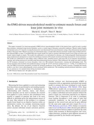
7. across a range of tasks, including a crossover cut (2A),
straight run (2B), eccentric FE at 60
/s (2C), and
concentric FE at 120
/s on a dynamometer (2D). Note
the ability of the model to predict both large and small
extension moments during the crossover cut and run
(2A and 2B, respectively). There was greater variation in
the shape and magnitude of the FE moments during the
dynamometer trials (Figs. 2C and D), although the
Table 3
Tendon slack lengths (Ltsj) for each muscle following calibration, the initial values prior to calibration (obtained using data from Lloyd and
Buchanan (1996)), and data from Delp (1990)
Tendon slack lengths for each subject (m)
Muscle 1 2 3 4 5 6 Mean S.D. Initial value Delp
SM 0.408 0.407 0.410 0.337 0.412 0.405 0.396 0.029 0.370 0.359
ST 0.262 0.288 0.301 0.280 0.265 0.278 0.279 0.015 0.265 0.262
BFL 0.360 0.403 0.405 0.372 0.379 0.373 0.382 0.018 0.360 0.341
BFS 0.247 0.243 0.246 0.241 0.285 0.248 0.252 0.017 0.250 0.100
SR 0.038 0.040 0.041 0.050 0.043 0.045 0.043 0.004 0.038 0.040
RF 0.332 0.338 0.335 0.330 0.324 0.334 0.332 0.005 0.311 0.346
TFL 0.390 0.393 0.394 0.378 0.395 0.375 0.387 0.009 0.391 0.425
GR 0.190 0.192 0.191 0.196 0.193 0.193 0.192 0.002 0.191 0.140
VM 0.108 0.117 0.118 0.116 0.107 0.111 0.113 0.005 0.112 0.126
VI 0.137 0.139 0.133 0.139 0.133 0.131 0.135 0.003 0.135 0.136
VL 0.148 0.153 0.157 0.158 0.148 0.149 0.152 0.005 0.156 0.157
MG 0.394 0.379 0.379 0.385 0.388 0.384 0.385 0.006 0.395 0.408
LG 0.370 0.353 0.358 0.389 0.387 0.386 0.374 0.016 0.365 0.385
-100
-50
0
50
100
150
200
0.2 0.4 0.6 0.8 1
time (s)
Moment(Nm)
-100
-50
0
50
100
150
200
0.2 0.4 0.6 0.8 1
time (s)
Moment(Nm)
R2
= 0.97
slope = 0.95
mre = 7.76
R2
= 0.94
slope = 0.91
mre = 4.86 Nm
Model prediction
Inverse dynamics
(A) Crossover Cut (B) Straight Run
-100
-50
0
50
100
150
200
0.4 0.8 1.2 1.6 2 2.4 2.8
time (s)
Moment(Nm)
-150
-100
-50
0
50
100
150
200
0.4 0.8 1.2 1.6 2 2.4 2.8
time (s)
Moment(Nm)
R2
= 0.89
slope = 0.94
mre = 7.76 Nm
R2
= 0.95
slope = 0.95
mre = 18.30 Nm
(C) Isokinetic dynamometer, eccentric
flexion/extension @ 60°/sec
(D) Isokinetic dynamometer, concentric
extension/flexion @ 120°/sec
Fig. 2. Comparison of model predictions of knee flexion/extension muscle moments and knee joint moments measured externally for subject 1.
Extension moments are positive on all graphs.
D.G. Lloyd, T.F. Besier / Journal of Biomechanics 36 (2003) 765–776 771

8. model was still able to predict the FE moments (mean
R2
¼ 0:7670:2). Temporal synchronisation of the mo-
ment data was maintained across all trials using the
40 ms delay in the EMG-to-Activation model (Eq. (1)).
The model also predicted FE joint moments in the
four subjects who returned for a repeat testing session
one week later, using the muscle model parameters from
the previous weeks’ calibration, but with re-calibration
of EMG-to-activation parameters. A one-way ANOVA
revealed that there were no significant differences in the
model predictions between different testing sessions
(Table 4).
Making the model less physiologically correct com-
promised the ability of the model to predict the inverse
dynamic joint moments. The predicted joint moment R2
significantly reduced from 0.91 to 0.85 (po0:001), when
model was re-calibrated with g ¼ 0%:
4. Discussion
Many studies have shown the promise of EMG-
driven musculoskeletal models to estimate muscle forces
and predict human joint moments over a limited set of
test data. The current model, following subject-specific
calibration, predicted the inverse dynamic FE knee joint
moments determined from a wide range of tasks and
different contractile conditions, thus supporting the
hypothesis of this study. The same muscle model
parameters were also used to give close predictions of
knee joint moments across different testing sessions,
which give confidence that the model and the subject-
specific parameters are representing the anatomy and
physiology of the system. The ability to predict gait
tasks as-well-as tasks performed using an isokinetic
dynamometer indicated that the model was not just
predicting moments for tasks that had similar patterns
of EMG and movement. The predictions were sensitive
to the physiological correctness of the model, where a
less physiologically correct model produced poorer
predictions. Finally, compared to previous EMG driven
models, the current model was better at predicting joint
moments calculated using inverse dynamics (Table 5).
Comparison of direct measures of muscle forces with
the EMG driven model estimates would be an ideal
method to validate the model. Unfortunately, ethical
Table 4
Model predictions across different testing sessions
Subject Session 1 Session 2
R2
R2
p
1 0.921 0.926 0.76
2 0.921 0.920 1.00
5 0.921 0.916 0.87
6 0.884 0.859 0.18
Table5
ComparisonofpreviousEMGdrivenmodelsandthecurrentdynamickneemodel
JointmodelledNo.ofsubjectsTotalno.
oftrials
Isometricor
dynamicmodel?
RangeoftasksperformedPredictions(R2
)
WhiteandWinter(1993)Hip,knee,andankle22DynamicCalibratedtodynamometer,testedduringgaitB0.79forknee
GranataandMarras(1995)Lowerback10703DynamicIsokineticandfreelifting0.81
NussbaumandChaffin(1998)Lowerback10398DynamicManualliftingandlowering0.76sagittalplane
Laursenetal.(1998)Shoulder6NAIsometricIsometricpushingandpulling0.74
LloydandBuchanan(1996)Knee7108IsometricIsometricflexion/extensionandvarus/valguscontractionsCV=17%
CurrentStudyKnee6204DynamicWiderangeofdynamometer,running,andcuttingtasks0.91
D.G. Lloyd, T.F. Besier / Journal of Biomechanics 36 (2003) 765–776772

9. and methodological considerations prevent in vivo
measures of muscle forces at the human knee. Inverse
dynamics calculations were used to calibrate the model
to an individual and as a means for an indirect
validation. This raises a question regarding the accuracy
of estimating joint moments using an inverse dynamics
approach. The FE moments, used to calibrate and
validate the model, are least susceptible to assumptions
associated with inverse dynamics calculations (e.g.
segmental inertial parameters—Pearsall and Costigan,
1999, and movement of markers—Holden et al., 1997).
The assumed FE axis of the knee may also influence the
inverse dynamics FE moments (Holden and Stanhope,
1998), however, the transepicondylar line as used in the
gait and isokinetic dynamometer trials in this study has
been shown to be a very good approximation of this axis
(Hollister et al., 1993; Churchill et al., 1998). Never-
theless it is difficult to speculate on the size of the error
in inverse dynamics FE moments estimated from the
gait trials because of the lack of a gold standard. In the
inverse dynamics calculations from the dynamometer
trials, the moment estimates were corrected for angular
acceleration of the limb and the dynamometer arm,
inline with the findings of Herzog (1988b). Thus
accurate measures of the FE torque (about 75%)
generated by the knee were expected from the dynam-
ometer trials (Herzog, 1988b).
It may be argued that this model represents nothing
more than a curve-fitting exercise that has no physio-
logical basis, given the number of parameters within the
model. However, there were only 18 free model
parameters that were adjusted in the calibration process
to fit 5 trials of data, with over 100 data points in each
trial (i.e. 18 parameters adjusted to fit over 500 data
points). In the data from the repeat experiments two
weeks later only 3 parameters were varied, for the same
number of calibration trials and data points. Moreover,
the calibrated models predicted on average about 30
trials of 100 points each for each subject. Thus the
model was very underdetermined. Additionally, the
curve-fitting argument could be raised if the adjustment
of model parameters were unconstrained. However,
there are many forms or levels of constraints inherent in
the construction of this model that ensures the model
represents the physiology and anatomy of the system.
Firstly, the mathematical constructs for the anatomy
and physiology constrain how elements in the model
behave. For example, the mathematical description of
the muscle and tendon model constrain how the muscles
generate force. Secondly, the calibration procedure
requires that the actual passive and active torque
generating capacity of the muscles are maintained for
each person. Thirdly, where muscle parameters required
adjustment, most changes were kept within bounds as
suggested in the literature. This was not the case for
tendon slack length as this has not been well established
in literature, but initial values where set on based
previous modelling work (Delp, 1990; Lloyd and
Buchanan, 1996) with adjustment permitted within a
small 715% range. Therefore, the constraints inherent
in this model greatly reduce the parameter solution
space that will allow good predictions of the net FE joint
moments.
It could be argued that the physiological correctness
of a model will have little effect on the accuracy of the
moment predictions as the calibration procedure makes
the model a simple curve fitting exercise. To this end, we
examined if the predictive ability of the model became
worse by removing the linear change in optimal fibre
length with activation, i.e. setting g ¼ 0% in Eq. (4). The
predicted joint moment R2
significantly reduced from
0.91 to 0.85 (po0:001). This result not only shows the
importance of modelling such physiologically phenom-
enon, but that the final calibrated model accuracy was
sensitive to the physiological correctness of the model,
i.e. the more physiological correct model gave better
predictions. It is anticipated that other physiological
phenomena will have to be included in future models to
better predict muscle behaviour at a macro level. For
example, incorporating non-linear changes in umax
with
the active state of muscle can easily be adapted to the
current model (Hatze, 1977). Similarly, history depen-
dence of muscle force (force depression/enhancement)
can also be added to the current model by linking
activation and previous mechanical work performed
within the contractile component (Herzog, 1998a;
Meijer et al., 1998), and may improve predictions in
the dynamometer trials.
There is still the possibility that the estimated muscle
forces are different to the actual muscle forces. This may
especially be true for muscles with small cross-sectional
area as these muscles’ contribution to the knee flexion/
extension moments are small relative to the larger
muscles (Lloyd and Buchanan, 2001), and the final
solution may not be very sensitive to change in the
smaller muscles’ parameters, i.e. tendon slack length.
This may not be a problem in the cases where EMG
driven models are used to estimate the load sharing
between ligaments and muscles, and joint contact forces,
as these are mostly determined by the activation and co-
contraction of the larger muscles (Lloyd and Buchanan,
2001). The predicted action of the larger muscles should
be closer to the actual muscle forces as the final joint
moments depend substantially on the action of these
muscles in the model. It is our experience that the model
needs all the large muscles acting in physiological
reasonable states for the model to predict both passive
joint torque and the joint moments in the maximally
activated trials. However, to ensure better estimation of
muscle forces future implementations of the model
should include a greater number of specifically chosen
calibration trials and physiological/anatomical measures
D.G. Lloyd, T.F. Besier / Journal of Biomechanics 36 (2003) 765–776 773

10. that will act to further constrain the solution space of
the model. For example, the larger prediction errors of
the dynamometer trials may have been due to only
having one active dynamometer trial within the calibra-
tion process. Therefore, increasing the number of
dynamometer trials within the calibration process may
constrain the parameter space to be more physiologi-
cally representative and achieve better overall predic-
tions. Systematically changing the hip and ankle joint
angles in some calibration dynamometer trails will
better constrain the solution of the two joint muscles
(Herzog and ter Keurs, 1988), thereby producing better
solutions for the single joint muscles.
A number of improvements can also be made to scale
the anatomical model of the lower limb to subjects’
anthropometry. The anatomical model used in this
study was a generic model of the lower limb based on
male cadaver data (Delp et al., 1990) and it was assumed
that the subjects were of similar anthropometric
proportions. For future modelling studies, a set of
scaling factors could be used (based on subject anthro-
pometric data) to alter the size and shape of bone and
muscle structures, as performed by Arnold et al. (2000).
This would allow for more representative estimations of
muscle tendon length and muscle moment arms for
individuals. It may also be possible to represent muscles
as multiple line segments to account for functionally
different segments of individual muscles. To differenti-
ate between mechanically functional different areas of
the muscles may also require information regarding the
activation of separate muscle segments and the use of
EMG electrode clusters. However, recently it has been
shown in the VL that very similar EMG-joint moment
relationships exist from quite different electrodes posi-
tions (Onishi et al., 2000).
Subject-specific optimal fibre lengths for each muscle
could also be included in the calibration process of the
dynamic knee model to account for changes in optimal
fibre length that may exist between different popula-
tions. Lloyd and Buchanan (1996) altered optimal fibre
lengths using a non-linear least squares parameter
calibration process in their isometric model. For the
purpose of this model, the optimal fibre lengths were set
to mean values determined by Lloyd and Buchanan
(1996), thereby reducing the number of variables in the
calibration process. Further calibration data may be
required if optimal fibre lengths are to be altered in the
calibration process so the model solution is suitably
constrained.
The 40 ms time delay used in the current model seems
to be an overestimate of the physiological electrome-
chanical delay, believed to be B10 ms (Corcos et al.,
1992). Future modelling attempts should reduce this
delay to 10 ms and account for temporal synchronisa-
tion of the joint moments by modelling the delay of
muscle force production within the musculotendon unit.
Following this, it is anticipated that the parameters in
the recursive EMG-to-activation model would be
adjusted differently to account for the temporal
synchronisation. This may also permit better predictions
of the FE moment data collected from the isokinetic
dynamometer.
The inclusion of muscle-specific activation parameters
will allow for individual linear or non-linear force–EMG
relationships (shape factor, A) for each muscle, which is
more appropriate physiologically (Woods and Bigland-
Ritchie, 1983), and may also result in better predictions
of muscle force and joint moments. For future studies,
the full parameter model (n ¼ 56) may be used with
genetic algorithms or simulated annealing to allow for
muscle specific EMG-to-Activation parameters to be
included in the model. Of course this will require a larger
set of calibration trials so the model solution is suitably
constrained.
It has been a point of discussion in the biomechanics
community regarding the apparent disagreement be-
tween isokinetic dynamometer and inverse dynamic
estimates of joint torque (see BIOMCH-L discussion on
Isokinetics and Inverse Dynamics by Devita, P., 1999).
However, in this study, the dynamic knee model
predicted FE moments for both the gait and isokinetic
dynamometer trials, albeit with a small reduction in
accuracy in the dynamometer trials. The ability to
predict both gait and dynamometer trials was because
the model included physiological means of increasing
force generating capacity of the muscles (i.e. eccentric
muscle action and storage of elastic energy in tendon via
stretch shorten cycle). Additionally, even though we
searched for the highest EMG during a number of MVC
trials at different knee angles, muscle activation in the
model could go above 1 in the any of the experimental
trials. Therefore inhibition of muscles during the
isometric MVC tasks could have occurred as has been
suggested by Suter and Herzog (1997) and was
accounted for. Further studies using such models could
help to identify the source of this apparent disagreement
between estimates of joint torque.
This paper has presented a generic EMG driven
musculoskeletal model using existing tools available to
the biomechanics community. This work has shown that
a non-linear least squares approach can be used with an
appropriate set of calibration data to obtain model
parameters that can be used in the musculoskeletal
model to predict inverse dynamic joint moments. The
model was cross validated across such a wide range of
tasks, whereas previous models have only been tested on
a limited set of tasks and better predicts these inverse
dynamic joint moments than previous models. A novel
approach was used to account for tissue filtering
characteristics and muscle activation dynamics. Impor-
tantly our work also showed that the more physiologi-
cally representative model gave better predictions.
D.G. Lloyd, T.F. Besier / Journal of Biomechanics 36 (2003) 765–776774

11. Further work will attempt to include other known
muscle contractile behaviour such as force depression/
enhancement, and individualised anatomical models.
Acknowledgements
The authors wish to acknowledge the support of the
National Health and Medical Research Council of
Australia (Grant #991134) and Musculographics Inc.
References
Aagaard, P., Simonsen, E.B., Beyer, N., Larsson, B., Magnusson, P.,
Kjaer, M., 1997. Isokinetic muscle strength and capacity for
muscular knee joint stabilization in elite sailors. International
Journal of Sports Medicine 18, 521–525.
Arnold, A.S., Salinas, S., Asakawa, D.J., Delp, S.L., 2000. Accuracy of
muscle moment arms estimated from MRI-based musculoskeletal
models of the lower extremity. Computer Aided Surgery 5,
108–119.
Besier, T.F., 1999. Examination of Neuromuscular and biomechanical
mechanisms of non-contact knee ligament injuries. Ph.D. Thesis,
University of Western Australia, Perth, Australia.
Besier, T.F., Lloyd, D.G., Cochrane, J.L., Ackland, T.R., 2001.
External loading of the knee joint during running and cutting
manoeuvres. Medicine and Science in Sports and Exercise 33,
1168–1175.
Brand, R.A., Pedersen, D.R., Friederich, J.A., 1986. The sensitivity of
muscle force predictions to changes in physiologic cross-sectional
area. Journal of Biomechanics 19, 589–596.
Brockett, C.L., Morgan, D.L., Proske, U., 2001. Human hamstring
muscles adapt to eccentric exercise by changing optimum length.
Medicine and Science in Sports and Exercise 33 (5), 783–790.
Buchanan, T.S., Lloyd, D.G., 1995. Muscle activity is different for
humans performing static tasks which require force control and
position control. Neuroscience Letters 194, 61–64.
Buchanan, T.S., Delp, S.L., Solbeck, J.A., 1998. Muscular resistance
to varus and valgus loads at the elbow. Journal of Biomechanical
Engineering 120, 634–639.
Churchill, D.L., Incavo, S.J., Johnson, C.C., Beynnon, B.D., 1998.
The transepicondylar axis approximates the optimal flexion axis of
the knee. Clinical Orthopaedics and Related Research 356,
111–118.
Corcos, D.M., Gottlieb, G.L., Latash, M.L., Almeida, G.L., Agarwal,
G.C., 1992. Electromechanical delay: an experimental artifact.
Journal of Electromyography and Kinesiology 2, 59–68.
Delp, S.L., 1990. A computer-graphics system to analyze and design
musculoskeletal reconstructions of the lower limb. Ph.D. Thesis,
Stanford University, CA.
Delp, S.L., Loan, J.P., 1995. A graphics-based software system to
develop and analyze models of musculoskeletal structures. Com-
puters in Biology and Medicine 25, 21–34.
Delp, S.L., Loan, J.P., Hoy, M.G., Zajac, F.E., Topp, E.L., Rosen,
J.M., 1990. An interactive graphics-based model of the lower
extremity to study orthopaedic surgical procedures. IEEE Transac-
tions on Biomedical Engineering 37, 757–767.
Epstein, M., Herzog, W., 1998. Theoretical Models of Skeletal Muscle.
Wiley, New York.
Fuglevand, A.J., Macefield, V.G., Bigland-Ritchie, B., 1999. Force–
frequency and fatigue properties of motor units in muscle that
control digits of the human hand. Journal of Neurophysiology 81,
1718–1729.
Fukunaga, T., Roy, R.R., Shellock, F.G., Hodgson, J.A., Edgerton,
V.R., 1996. Specific tension of human plantar flexors and
dorsiflexors. Journal of Applied Physiology 80, 158–165.
Gordon, A.M., Huxley, A.F., Julian, F.J., 1966. The variation in
isometric tension with sarcomere length in vertebrate muscle fibres.
Journal of Physiology 184, 170–192.
Granata, K.P., Marras, W.S., 1993. An EMG-assisted model of loads
on the lumbar spine during asymmetric trunk extensions. Journal
of Biomechanics 26, 1429–1438.
Granata, K.P., Marras, W.S., 1995. An EMG-assisted model of trunk
loading during free-dynamic lifting. Journal of Biomechanics 28,
1309–1317.
Guimaraes, A.C., Herzog, W., Hulliger, M., Zhang, Y.T., Day, S.,
1994. Effects of muscle length on the EMG-force relationship of
the cat soleus muscle studied using non-periodic stimulation of
ventral root filaments. Journal of Experimental Biology 193, 49–64.
Guimar*aes, A.C., Herzog, W., Allinger, T.L., Zhang, Y.T., 1995. The
EMG–force relationship of the cat soleus muscle and its associa-
tion with contractile conditions during locomotion. Journal of
Experimental Biology 198, 975–987.
Hatze, H., 1977. A myocybernetic control model of skeletal muscle.
Biological Cybernetics 25, 103–119.
Hatze, H., 1981. Estimation of myodynamic parameter values from
observations on isometrically contracting muscle groups. European
Journal of Applied Physiology 46, 325–338.
Hayes, K.W., Falconer, J., 1992. Differential muscle strength decline in
osteoarthritis of the knee. A developing hypothesis. Arthritis Care
Research 5, 24–28.
Herzog, W., 1998a. History dependence of force production in skeletal
muscle: a proposal for mechanisms. Journal of Electromyography
and Kinesiology 8, 111–117.
Herzog, W., 1988b. The relation between the resultant moments at a
joint and the moments measured by an isokinetic dynamometer.
Journal of Biomechanics 21, 5–12.
Herzog, W., ter Keurs, H.E., 1988. A method for the determination of
the force–length relation of selected in-vivo human skeletal
muscles. European Journal of Physiology 411, 637–641.
Herzog, W., Guimaraes, A.C., Anton, M.G., Carter-Erdman, K.A.,
1991. Moment-length relations of rectus femoris muscles of speed
skaters/cyclists and runners. Medicine and Science in Sports and
Exercise 23, 1289–1296.
Herzog, W., Sokolosky, J., Zhang, Y.T., Guimaraes, A.C., 1998.
EMG–force relation in dynamically contracting cat plantaris
muscle. Journal of Electromyography and Kinesiology 8, 147–155.
Hof, A.L., van den Berg, J.W., 1981a. EMG-to-force processing. II.
Estimation of parameters of the Hill Muscle model for the human
triceps surae by means of calf ergometer. Journal of Biomechanics
14, 759–770.
Hof, A.L., van den Berg, J.W., 1981b. EMG-to-force processing. III.
Estimation of model parameters for the human triceps surae
muscle and the assessment of the accuracy by means of a torque
plate. Journal of Biomechanics 14, 771–785.
Holden, J.P., Stanhope, S.J., 1998. The effect of variation in knee
center location estimates on net knee joint moments. Gait and
Posture 7, 1–6.
Holden, J.P., Orsini, J.A., Lohmann Siegel, K., Kepple, T.M., Gerber,
L.H., Stanhope, S.J., 1997. Surface movement errors in shank
kinematics and knee kinetics during gait. Gait and Posture 5,
217–227.
Hollister, A.M., Jatana, S., Singh, A.K., Sullivan, W.W., Lupichuk,
A.G., 1993. The axes of rotation of the knee. Clinical Orthopaedics
and Related Research 290, 259–268.
Huijing, P.A., 1996. Important experimental factors for skeletal muscle
modelling: non-linear changes of muscle length force characteristics
as a function of degree of activity. European Journal of
Morphology 34, 47–54.
D.G. Lloyd, T.F. Besier / Journal of Biomechanics 36 (2003) 765–776 775

12. Kadaba, M.P., Ramakrishnan, H.K., Wootten, M.E., 1990. Measure-
ment of lower extremity kinematics during level walking. Journal
of Orthopaedic Research 8, 383–392.
Laursen, B., Jenson, B., Nemeth, G., Sjogaard, G., 1998. A model
predicting individual shoulder muscle forces based on relationship
between electromyographic and 3D external forces in static
position. Journal of Biomechanics 31, 731–739.
Lloyd, D.G., Buchanan, T.S., 1996. A model of load sharing between
muscles and soft tissues at the human knee during static tasks.
Journal of Biomechanical Engineering 118, 367–376.
Lloyd, D.G., Buchanan, T.S., 2001. Strategies of muscular support of
varus and valgus isometric loads at the human knee. Journal of
Biomechanics 34, 1257–1267.
Lloyd, D.G., Gonzalez, R.V., Buchanan, T.S., 1996. A general EMG-
driven musculoskeletal model for prediction of human joint
moments. Paper Presented at the Australian Conference of Science
and Medicine in Sport, Australia.
Loan, P.J., 1992. Dynamics Pipeline. Evanston IL, Musculographics.
McGill, S.M., 1992. A myoelectrically based dynamic three-dimen-
sional model to predict loads on lumbar spine tissues during lateral
bending. Journal of Biomechanics 25, 395–414.
McGill, S.M., Norman, R.W., 1986. Partitioning of the L4-L5
dynamic moment into disc, ligamentous, and muscular components
during lifting. Spine 11, 666–678.
Meijer, K., Grootenboer, H.J., Koopman, H.F.J.M., van der Linden,
B.J.J.J., Huijing, P.A., 1998. A hill type model of rat medial
gastrocnemius muscle that accounts for shortening history effects.
Journal of Biomechanics 31, 555–563.
Milner-Brown, H.S., Stein, R.B., Yemm, R., 1973. Changes in firing
rate of human motor units during linearly changing voluntary
contractions. Journal of Physiology (London) 228, 371–390.
Nussbaum, M., Chaffin, D., 1998. Lumbar muscle force estimation
using a subject-invariant 5-parameter EMG-based model. Journal
of Biomechanics 31, 667–672.
Onishi, H., Yagi, R., Akasaka, K., Momose, K., Ihashi, K., Handa,
Y., 2000. Relationship between EMG signals and force in human
vastus lateralis using multiple bipolar wire electrodes. Journal of
Electromyography and Kinesiology 10, 59–67.
Pearsall, D.J., Costigan, P.A., 1999. The effect of segment parameter
error on gait analysis results. Gait and Posture 9, 173–183.
Piazza, S.J., Delp, S.L., 1996. The influence of muscles on knee flexion
during the swing phase of gait. Journal of Biomechanics 29,
723–733.
Potvin, J.R., Norman, R.W., McGill, S.M., 1996. Mechanically
corrected EMG for the continuous estimation of erector spinae
muscle loading during repetitive lifting. European Journal of
Applied Physiology and Occupational Physiology 74, 119–132.
Rabiner, L.R., Gold, B., 1975. Theory and application of digital signal
processing. Englewood Cliffs, NJ, USA, Prentice Hall.
Read, M.T., Bellamy, M.J., 1990. Comparison of hamstring/quad-
riceps isokinetic strength ratios and power in tennis, squash
and track athletes. British Journal of Sports Medicine 24,
178–182.
Schutte, L.M., 1992. Using musculoskeletal models to explore
strategies for improving performance in electrical stimulation-
induced leg cycle ergometry. Ph.D. Thesis, Stanford University.
Schutte, L.M., Rodgers, M.M., Zajac, F.E., 1993. Improving the
efficacy of electrical simulation-induced leg cycle ergometry: an
analysis based on a dynamic musculoskeletal model. IEEE
Transactions on Rehabilitation Engineering 1, 109–125.
Scott, S.H., Winter, D.A., 1991. A comparison of three muscle
pennation assumptions and their effect on isometric and isotonic
force. Journal of Biomechanics 24, 163–167.
Soechting, J.F., Flanders, M., 1997. Evaluating an integrated
musculoskeletal model of the human arm. Journal of Biomecha-
nical Engineering 119, 93–102.
Suter, E., Herzog, W., 1997. Extent of muscle inhibition as a function
of knee angle. Journal of Electromyography and Kinesiology 7,
123–130.
Tax, A.A., Denier van der Gon, J.J., Erkelens, C.J., 1990. Differences
in coordination of elbow flexor muscles in force tasks and
movement tasks. Experimental Brain Research 81, 567–572.
Thelen, D.G., Schultz, A.B., Fassois, S.D., Ashton-Miller, J.A., 1994.
Identification of dynamic myoelectric signal-to-force models during
isometric lumbar muscle contractions. Journal of Biomechanics 27,
907–919.
Van Ruijven, L.J., Weijs, W.A., 1990. A new model for calculating
muscle forces from electromyograms. European Journal of Applied
Physiology and Occupational Physiology 61, 479–485.
White, S.C., Winter, D.A., 1993. Predicting muscle forces in gait from
EMG signals and musculotendon kinematics. Journal of Electro-
myography and Kinesiology 2, 217–231.
Woods, J.J., Bigland-Ritchie, B., 1983. Linear and non-linear surface
EMG/force relationships in human muscles. An anatomical/
functional argument for the existence of both. American Journal
of Physical Medicine 62, 287–299.
Yamaguchi, G.T., Sawa, A.G.U., Moran, D.W., Fessler, M.J.,
Winters, J.M., 1990. A survey of human musculotendon actuator
parameters. In: Winters, J.M., Woo, S.L-Y. (Eds.), Multiple
Muscle Systems: Biomechanics and Movement Organization.
Springer, New York, pp. 717–773.
Zajac, F.E., 1989. Muscle and tendon: properties, models, scaling, and
application to biomechanics and motor control. Critical Reviews in
Biomedical Engineering 17, 359–411.
D.G. Lloyd, T.F. Besier / Journal of Biomechanics 36 (2003) 765–776776