1. A Novel Muscle Coordination Method
for Musculoskeletal Humanoid Systems
and Its Application in Bionic Arm Control
Haiwei Dong1
and Setareh Yazdkhasti2
1
Devision of Engineering, New York University AD, Electra Street, Abu Dhabi, UAE
haiwei.dong@nyu.edu
2
College of Engineering, Al Ghurair University, Academic City, Dubai, UAE
s.yazdkhasti@ieee.org
Abstract. The muscle force control of musculoskeletal humanoid sys-
tem has been considered for years in motor control, biomechanics and
robotics disciplines. In this paper, we consider the muscle force control as
a problem of muscle coordination. We give a general muscle coordination
method for mechanical systems driven by agonist and antagonist muscles.
Specifically, the muscle force is computed by two steps. First, the initial
muscle force is computed by pseudo-inverse. Here, the pseudo-inverse
solution naturally satisfies the minimum total muscle force in the least
squares sense. Second, the initial optimized muscle force is optimized by
taking the optimization criteria of distributing muscle force in the mid-
dle of its output force range. The two steps provide an even-distributed
muscle force. The proposed method is validated by a movement tracking
of a bionic arm which has 5 degrees of freedom and 22 muscles. The force
distribution property, tracking accuracy and efficiency are also tested.
Keywords: Muscle Force Computation, Arm Movement Control, Re-
dundancy Solution.
1 Introduction
Several research works in different disciplines have been distributed in order to
understand the muscle control of the musculoskeletal humanoid systems. The
initial scientific works in human motor control consider the muscle control as
coordination of sensor input and motor output. The sensor-motor coordination
is explained by modeled central nervous system [1]. Later, the muscle control is
dealt with in biomechanics. Here, the basic idea is building an accurate muscle
model, setting all the constraints in muscle space and joint space (such as force
limit, motion boundary, time delay etc.) and using global optimization to solve
the problem as a whole [2][3]. As the global optimization is computationally very
exhaustive task, parallel computation is introduced to reduce the computational
time [4]. There have been two successful commercial software packages to simu-
late human movement: AnyBody Modeling System by AnyBody Technology and
SIMM by MusculoGraphics. Recently, with the development of artificial muscle
M. Lee et al. (Eds.): ICONIP 2013, Part I, LNCS 8226, pp. 233–240, 2013.
c Springer-Verlag Berlin Heidelberg 2013

2. 234 H. Dong and S. Yazdkhasti
technology, many muscle-like actuators are available, such as cable-driven ac-
tuator, pneumatic actuator, and so on. By using these new actuators, robotic
researchers built a number of musculoskeletal humanoid robots, such as ECCE
from University of Zurich, Kenshiro from University of Tokyo, Lucy from Vrije
Universiteit Brussel, etc. These robots provide physical platforms to emulate
muscle force control of musculoskeletal systems. However, the control of these
musculoskeletal humanoid system is still under development. Regarding the co-
incidence with electromyogram (EMG) measurement, there has been one paper
written by Anderson and Pandy, stating that the muscle force curve computed
by the global optimization looks similar with the real EMG measurement when
doing extreme movement of high jumping [4].
Actually, the muscle force control can be considered as muscle coordination.
As there exists redundancy in joint space, muscle space and impedance space, the
solution of the muscle coordination is not unique [5]. Based on different criteria,
the muscle coordination solutions are different. For example, Pandy considered
the criterion of the minimum of the overall energy-consuming of muscles[3]. Dong
et al. chose the criterion to be “anti-fatigue”, i.e., the load was distributed evenly
among muscles [6]. If we only focus on the control performance without consid-
ering energy-consuming or force distribution, the problem is easier. In Tahara
et al.’s research, the muscle force is distributed from computed joint torque. PD
control is then used for each muscle’s control [7]. Actually, from the neuroscience
research, the muscle force control is also influenced by the body movement pat-
terns. The dynamics of the musculoskeletal system has order parameter which
can determine the phase transition of movements. These scenarios are found in
finger movement and limb movement patterns [8].
In this paper, we give a general muscle coordination method for mechanical
systems driven by agonist and antagonist muscles. Specifically, the muscle force
is computed by two steps. First, the initial muscle force is computed by pseudo-
inverse. Here, the pseudo-inverse solution naturally satisfies the minimum total
muscle force in the least squares sense. Second, the initial optimized muscle force
is optimized by taking the optimization criteria of distributing muscle force in
the middle of its output force range. The two steps provide an even-distributed
muscle force. The proposed method is validated by a movement tracking of a
bionic arm which has 5 degrees of freedom and 22 muscles. The force distribution
property, tracking accuracy and efficiency are also tested.
2 Muscle Coordination
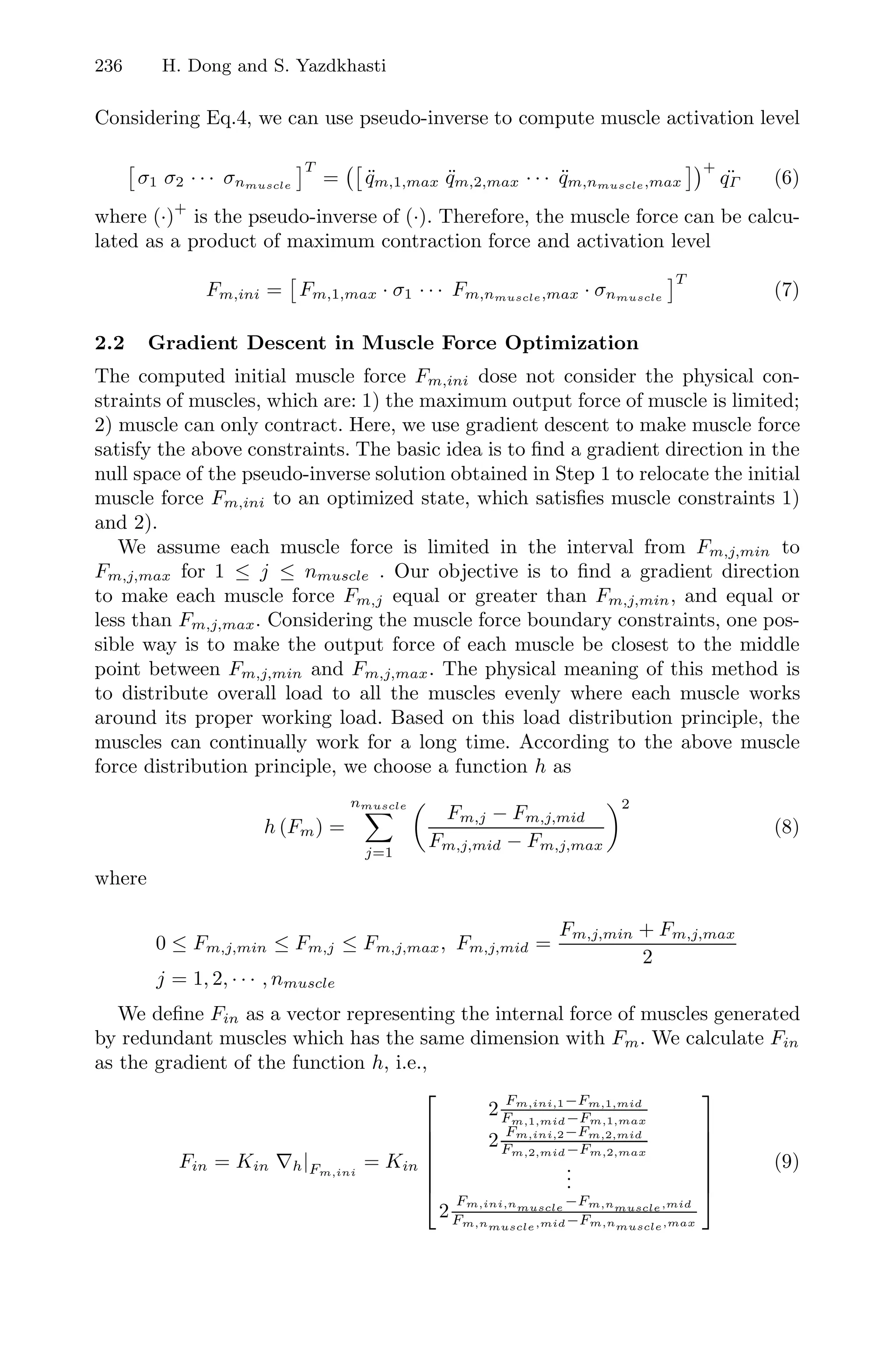
2.1 Pseudo-inverse in Initial Muscle Force Computation
In this subsection, we use pseudo-inverse to compute the initial muscle force.
The input is the desired joint trajectory and muscle force boundary. The output
is the minimum muscle force under the sense of least-squares. The basic idea
is firstly creating a linear equation based on the description of the acceleration
contribution in joint space and muscle space, respectively. Then the muscle acti-
vation level is calculated by solving the above linear equation. Finally, the muscle

3. A Novel Muscle Coordination Method and Its Application 235
force is computed by scaling the muscle activation level with its corresponding
maximum muscle force.
The general dynamic equation of the musculoskeletal systems can be written
in the general form
H (q, t) ¨q + C (q, t) ˙q + G (t) = f (Fm) (1)
where f (Fm) maps muscle force Fm to joint torque. Here, we transform it into
the following form
¨q = H (q, t)
−1
f (Fm)
¨qΓ
+ −H (q, t)
−1
(C (q, t) + G (t))
¨qΛΞ
(2)
The above equations indicate that in the joint space, the acceleration contri-
bution comes from 1): joint torque Γ, 2): centripetal, coriolis and gravity torque
Λ + Ξ. Hence, we can compute the acceleration contribution from joint torque
¨qΓ by Eq.2. Whereas, from another viewpoint, in the muscle space, each muscle
has its acceleration contribution. Here, we assume the total muscle number is
nmuscle. For the j-th (1 ≤ j ≤ nmuscle) muscle, its maximum acceleration con-
tribution can be written as
¨qm,j,max = H (q, t)−1
Γj,max (1 ≤ j ≤ nmuscle) (3)
where
Γ1,max = JT
m Fm,1,max 0 0 · · · 0 0
T
Γ2,max = JT
m 0 Fm,2,max 0 · · · 0 0
T
· · ·
Γnmuscle,max = JT
m 0 0 0 · · · 0 Fm,nmuscle,max
T
By combining the above two computational ways of acceleration contribution
in joint space and muscle space, we can build a linear equation
¨qm,1,max ¨qm,2,max · · · ¨qm,nmuscle,max σ1 σ2 · · · σnmuscle
T
= ¨qΓ (4)
where σ1 σ2 · · · σnmuscle
T
is a vector of muscle activation levels. The muscle
activation level is a scalar in the interval [0, 1], representing the percentage of
maximum contraction force of muscle. It is noted that ¨qm,j,max (1 ≤ j ≤ nmuscle)
and ¨qΓ are vectors. The dimensions of ¨qm,j,max and ¨qΓ are the same equaling to
the joint number. Supposing the total joint number is njoint, ¨qm,j,max and ¨qΓ
can be written in the form
¨qm,j,max =
⎡
⎢
⎢
⎢
⎣
¨qm,j,1
¨qm,j,2
...
¨qm,j,njoint
⎤
⎥
⎥
⎥
⎦
njoint×1
, ¨qΓ =
⎡
⎢
⎢
⎢
⎣
¨qΓ,1
¨qΓ,2
...
¨qΓ,njoint
⎤
⎥
⎥
⎥
⎦
njoint×1
(5)

4. 236 H. Dong and S. Yazdkhasti
Considering Eq.4, we can use pseudo-inverse to compute muscle activation level
σ1 σ2 · · · σnmuscle
T
= ¨qm,1,max ¨qm,2,max · · · ¨qm,nmuscle,max
+
¨qΓ (6)
where (·)+
is the pseudo-inverse of (·). Therefore, the muscle force can be calcu-
lated as a product of maximum contraction force and activation level
Fm,ini = Fm,1,max · σ1 · · · Fm,nmuscle,max · σnmuscle
T
(7)
2.2 Gradient Descent in Muscle Force Optimization
The computed initial muscle force Fm,ini dose not consider the physical con-
straints of muscles, which are: 1) the maximum output force of muscle is limited;
2) muscle can only contract. Here, we use gradient descent to make muscle force
satisfy the above constraints. The basic idea is to find a gradient direction in the
null space of the pseudo-inverse solution obtained in Step 1 to relocate the initial
muscle force Fm,ini to an optimized state, which satisfies muscle constraints 1)
and 2).
We assume each muscle force is limited in the interval from Fm,j,min to
Fm,j,max for 1 ≤ j ≤ nmuscle . Our objective is to find a gradient direction
to make each muscle force Fm,j equal or greater than Fm,j,min, and equal or
less than Fm,j,max. Considering the muscle force boundary constraints, one pos-
sible way is to make the output force of each muscle be closest to the middle
point between Fm,j,min and Fm,j,max. The physical meaning of this method is
to distribute overall load to all the muscles evenly where each muscle works
around its proper working load. Based on this load distribution principle, the
muscles can continually work for a long time. According to the above muscle
force distribution principle, we choose a function h as
h (Fm) =
nmuscle
j=1
Fm,j − Fm,j,mid
Fm,j,mid − Fm,j,max
2
(8)
where
0 ≤ Fm,j,min ≤ Fm,j ≤ Fm,j,max, Fm,j,mid =
Fm,j,min + Fm,j,max
2
j = 1, 2, · · · , nmuscle
We define Fin as a vector representing the internal force of muscles generated
by redundant muscles which has the same dimension with Fm. We calculate Fin
as the gradient of the function h, i.e.,
Fin = Kin ∇h|Fm,ini
= Kin
⎡
⎢
⎢
⎢
⎢
⎢
⎣
2
Fm,ini,1−Fm,1,mid
Fm,1,mid−Fm,1,max
2
Fm,ini,2−Fm,2,mid
Fm,2,mid−Fm,2,max
...
2
Fm,ini,nmuscle
−Fm,nmuscle,mid
Fm,nmuscle,mid−Fm,nmuscle,max
⎤
⎥
⎥
⎥
⎥
⎥
⎦
(9)

5. A Novel Muscle Coordination Method and Its Application 237
where Kin is a scalar matrix controlling the optimization speed. It is easy to
prove that the direction of Fin points to Fm,i,mid. We map the internal force Fin
into Fm space (i.e., pseudo-inverse solution’s null space) as
g (Fin) = I − JT
m
+
JT
m Fin (10)
where I is an identity matrix having the same dimension with muscle space.
According to Moore-Penrose pseudo-inverse, g (Fin) is orthogonal with the space
of Fm,ini. Finally, the optimized muscle force is calculated as
Fm = Fm,ini + g (Fin) (11)
3 Evaluation
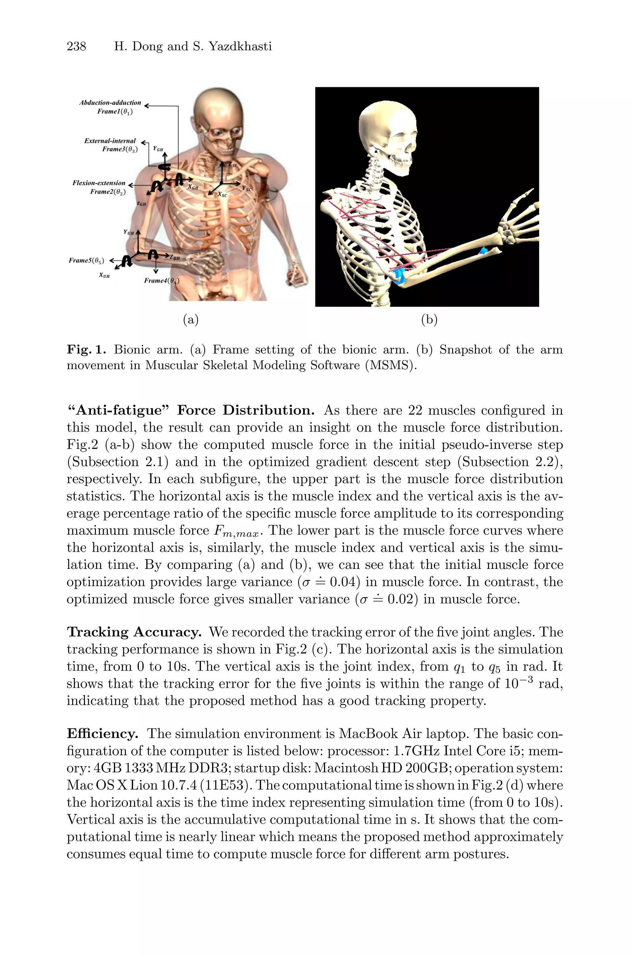
3.1 Bionic Arm Modeling
First of all, we define symbols for the convenience of derivation. Rot(θ, x),
Rot(θ, y) and Rot(θ, z) are rotation matrices between different frames x, y, and z
axis where θ is the rotation angle. T rans(dx, dy, dz) is transition matrix within a
frame where dx, dy, and dz are the transition distances in x, y, and z directions,
respectively. T j
i is the transfer matrix from frame i to frame j. In this simulation,
we defined the frame 1 to 5 as shown in Fig.1 (a). Joint angles [θ1, θ2, θ3, θ4, θ5]T
are the rotational angles corresponding to Frame 1 to Frame 5, respectively. The
range of shoulder angle is set as from -20 to 100 degrees, and the range of the
elbow is set as from 0 to 170 degrees. Here, we use Muscular Skeletal Modeling
Software (MSMS) [9] to create the virtual bionic arm, based on which, we make
animation to evaluate the movement computed by the proposed method (Fig.1
(b)).
In the simulation, the bionic arm is composed of two parts: shoulder and el-
bow. In total, the model is composed of five rotational degrees of freedom (DOF)
where three of them are in the shoulder joint (shoulder abduction-adduction,
shoulder flexion-extension and shoulder external-internal rotation), and two are
in the elbow joint (elbow flexion-extension and forearm pronation-supination).
The parameters setting of the bionic arm is based on the real data of a human
upper limb. The setting of length, mass, mass center position and inertia coeffi-
cients are from [10]. There are 22 muscles configured in the model. The specific
configuration of the muscles, i.e., coordinate setting of the origins and insertions
in the Gleno-Humeral joint coordinate system (XGH, YGH, ZGH), are from [11].
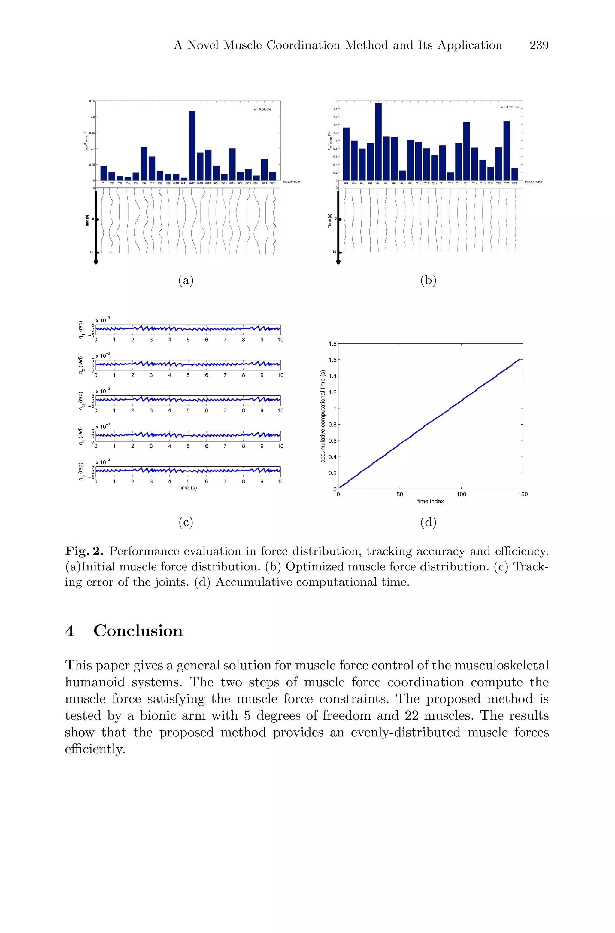
3.2 Performance
We used the above bionic arm model to test the proposed method. Without loss
of generality, the desired trajectory of the five rotational joints is sine signal:
amplitude: -1/3π; frequency: 1; phase: 0; bias: 1/3π. The maximum muscle force
Fm,i,max (1 ≤ i ≤ 22) is set as 100N. The total simulation time is set as 10s.

6. 238 H. Dong and S. Yazdkhasti
(a) (b)
Fig. 1. Bionic arm. (a) Frame setting of the bionic arm. (b) Snapshot of the arm
movement in Muscular Skeletal Modeling Software (MSMS).
“Anti-fatigue” Force Distribution. As there are 22 muscles configured in
this model, the result can provide an insight on the muscle force distribution.
Fig.2 (a-b) show the computed muscle force in the initial pseudo-inverse step
(Subsection 2.1) and in the optimized gradient descent step (Subsection 2.2),
respectively. In each subfigure, the upper part is the muscle force distribution
statistics. The horizontal axis is the muscle index and the vertical axis is the av-
erage percentage ratio of the specific muscle force amplitude to its corresponding
maximum muscle force Fm,max. The lower part is the muscle force curves where
the horizontal axis is, similarly, the muscle index and vertical axis is the simu-
lation time. By comparing (a) and (b), we can see that the initial muscle force
optimization provides large variance (σ
.
= 0.04) in muscle force. In contrast, the
optimized muscle force gives smaller variance (σ
.
= 0.02) in muscle force.
Tracking Accuracy. We recorded the tracking error of the five joint angles. The
tracking performance is shown in Fig.2 (c). The horizontal axis is the simulation
time, from 0 to 10s. The vertical axis is the joint index, from q1 to q5 in rad. It
shows that the tracking error for the five joints is within the range of 10−3
rad,
indicating that the proposed method has a good tracking property.
Efficiency. The simulation environment is MacBook Air laptop. The basic con-
figuration of the computer is listed below: processor: 1.7GHz Intel Core i5; mem-
ory: 4GB 1333 MHz DDR3; startup disk: Macintosh HD 200GB; operation system:
Mac OS X Lion 10.7.4 (11E53). The computational time is shown in Fig.2 (d) where
the horizontal axis is the time index representing simulation time (from 0 to 10s).
Vertical axis is the accumulative computational time in s. It shows that the com-
putational time is nearly linear which means the proposed method approximately
consumes equal time to compute muscle force for different arm postures.

7. A Novel Muscle Coordination Method and Its Application 239
(a) (b)
0 1 2 3 4 5 6 7 8 9 10
−5
0
5
x 10
−3
q
1
(rad)
0 1 2 3 4 5 6 7 8 9 10
−5
0
5
x 10
−3
q
2
(rad)
0 1 2 3 4 5 6 7 8 9 10
−5
0
5
x 10
−3
q
3
(rad)
0 1 2 3 4 5 6 7 8 9 10
−5
0
5
x 10
−3
q
4
(rad)
0 1 2 3 4 5 6 7 8 9 10
−5
0
5
x 10
−3
time (s)
q
5
(rad)
(c)
0 50 100 150
0
0.2
0.4
0.6
0.8
1
1.2
1.4
1.6
1.8
time index
accumulativecomputationaltime(s)
(d)
Fig. 2. Performance evaluation in force distribution, tracking accuracy and efficiency.
(a)Initial muscle force distribution. (b) Optimized muscle force distribution. (c) Track-
ing error of the joints. (d) Accumulative computational time.
4 Conclusion
This paper gives a general solution for muscle force control of the musculoskeletal
humanoid systems. The two steps of muscle force coordination compute the
muscle force satisfying the muscle force constraints. The proposed method is
tested by a bionic arm with 5 degrees of freedom and 22 muscles. The results
show that the proposed method provides an evenly-distributed muscle forces
efficiently.

8. 240 H. Dong and S. Yazdkhasti
References
1. Wise, S., Shadmehr, R.: Motor Control. In: Encyclopedia of the Human Brain, pp.
137–157 (2002)
2. Garner, B.A., Pandy, M.G.: A kenematic model of the upper limb based on the
visible human project (vhp) image dataset. Computer Methods in Biomechanics
and Biomedical Engineering 2, 107–124 (1999)
3. Pandy, M.: Computer modeling and simulation of human movement. Annual Re-
view of Biomedical Engineering 3, 245–273 (2001)
4. Anderson, F., Pandy, M.: A dynamic optimization solution for vertical jumping in
three dimensions. Computer Methods in Biomechanics and Biomedical Engineer-
ing 2, 201–231 (1999)
5. Yamaguchi, G.: Dynamic Modeling of Musculoskeletal Motion: A Vectorized Ap-
poach for Biomechanical Analysis in Three Dimensions. Springer (2005)
6. Dong, H., Mavridis, N.: Muscle force distribution for adaptive control of a hu-
manoid robot arm with redundant bi-articular and mono-articular muscle mecha-
nism. Artificial Life and Robotics (2013)
7. Tahara, K., Luo, Z., Arimoto, S., Kino, H.: Sensory-motor control mechanism for
reaching movements of a redundant musculo-skeletal arm. Journal of Robotic Sys-
tems 22, 639–651 (2005)
8. Kelso, J.A.: Dynamic Patterns. MIT Press (1995)
9. Khachani, M., Davoodi, R., Loeb, G.: Musculo-skeletal modeling software (msms)
for biomechanics and virtual rehabilitation. In: Proceeding of American Society of
Biomechanics Conference (2007)
10. Nagano, A., Yoshioka, S., Komura, T., Himeno, R., Fukashiro, S.: A three-
dimensional linked segment model of the whole human body. International Journal
of Sport and Health Science 3, 311–325 (2005)
11. Maurel, W., Thalmann, D., Hoffmeyer, P., Beylot, P., Gingins, P., Kalra, P., Mag-
nenat, N., Hoffmeyer, P.: A biomechanical musculoskeletal model of human upper
limb for dynamic simulation. In: Proceedings of the Eurographics Computer Ani-
mation and Simulation Workshop (1996)