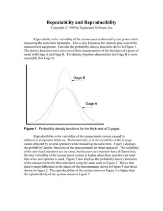
This document discusses repeatability and reproducibility in measurement systems. Repeatability refers to the variability from measurements taken by the same person on the same item, and depends on the precision of the measurement equipment. Reproducibility refers to variability from measurements taken by different operators on the same item. The document provides examples of using the range-and-average method and analysis of variance (ANOVA) method to quantify repeatability, reproducibility, and overall measurement system variability.
Sparse Representation for Fetal QRS Detection in Abdominal ECG RecordingsRiccardo Bernardini
Slideshow of the presentation given at EHB 2015
In this work, we consider the problem of detection of fetal heart beats from abdominal, non-invasive mixture recordings. We propose a new method for the separation of maternal and fetal beats based on the sparse decomposition in an over-complete dictionary of Gaussian-like functions. To increase the detection capability, we also use Independent Component Analysis (ICA) after maternal template subtraction. We show that the proposed detection method can be applied on the original mixture with a sensitivity close to 95%. Moreover, our method may be used also for single channel abdominal ECG signals, and also used in real-time applications.
Lower back pain can be caused by a variety of problems with any parts of the complex, interconnected network of spinal muscles, nerves, bones, discs or tendons in the lumbar spine. This solution is about to identify a person is abnormal or normal using collected physical spine details.
Kano GIS Day 2014 - The Application of Multivariate Geostatistical analyses i...eHealth Africa
We are excited to be holding our own GIS Day event on November 19th, 2014!
GIS Day is a global grassroots educational event that enables Geographic Information Systems (GIS) users and vendors to showcase real-world applications of GIS to schools, businesses, and the general public. Organizations that utilize GIS around the world participate by holding or sponsoring an event of their own.
The first formal GIS Day took place in 1999. In 2005, more than 700 GIS Day events were held in 74 countries around the globe. Esri president and co-founder Jack Dangermond credits Ralph Nader with inspiring the creation of GIS Day. He saw GIS Day as providing an opportunity for the world to learn about the uses of GIS in mapping geography, and what that mapping technology could provide. He wanted GIS Day to be a grassroots effort and open to everyone to participate.
Recognizing the power that GIS technology could provide for healthcare, eHealth Africa as an NGO organization stepped to the forefront of using GIS applications to track polio in Nigeria. Using GIS technology, eHealth is able to map out areas previously unreached during immunization campaigns. Once the area is mapped, much-needed polio vaccinations are able to be distributed and the polio epidemic is brought another step closer to being controlled and eliminated.
The theme of GIS Day is “Discovering the world through GIS.” GIS Day provides an international forum for users of GIS technology to demonstrate real-world applications that are making a difference in our society and around the world.
We are excited to take part in GIS Day 2014 on November 19th. We look forward to joining with our community partners in discussing GIS usage, and to take a close look at the exciting contributions GIS provides around our world.
Measurement systems analysis and a study of anova methodeSAT Journals
Abstract
Instruments and measurement systems form the base of any process improvement strategies. The much widely used QC tools like
SPC depends on sample data taken from processes to track process variation which in turn depends on measuring system itself.
The purpose of Measurement System Analysis is to qualify a measurement system for use by quantifying its accuracy, precision,
and stability and to minimize their contribution in process variation through inherent tools such as ANOVA. The purpose of this
paper is to outline MSA and study ANOVA method through a real-time shop floor experiment.
Keywords: SPC, Accuracy, Precision, Stability, QC, ANOVA
Detailed illustration of MSA procedures both for Variable and attribute, Analysis of results and planning for MSA. Complete guidance for planning and implementation of MSA.
Vaccine management system project report documentation..pdfKamal Acharya
The Division of Vaccine and Immunization is facing increasing difficulty monitoring vaccines and other commodities distribution once they have been distributed from the national stores. With the introduction of new vaccines, more challenges have been anticipated with this additions posing serious threat to the already over strained vaccine supply chain system in Kenya.
Water scarcity is the lack of fresh water resources to meet the standard water demand. There are two type of water scarcity. One is physical. The other is economic water scarcity.
Event Management System Vb Net Project Report.pdfKamal Acharya
In present era, the scopes of information technology growing with a very fast .We do not see any are untouched from this industry. The scope of information technology has become wider includes: Business and industry. Household Business, Communication, Education, Entertainment, Science, Medicine, Engineering, Distance Learning, Weather Forecasting. Carrier Searching and so on.
My project named “Event Management System” is software that store and maintained all events coordinated in college. It also helpful to print related reports. My project will help to record the events coordinated by faculties with their Name, Event subject, date & details in an efficient & effective ways.
In my system we have to make a system by which a user can record all events coordinated by a particular faculty. In our proposed system some more featured are added which differs it from the existing system such as security.
Saudi Arabia stands as a titan in the global energy landscape, renowned for its abundant oil and gas resources. It's the largest exporter of petroleum and holds some of the world's most significant reserves. Let's delve into the top 10 oil and gas projects shaping Saudi Arabia's energy future in 2024.
Courier management system project report.pdfKamal Acharya
It is now-a-days very important for the people to send or receive articles like imported furniture, electronic items, gifts, business goods and the like. People depend vastly on different transport systems which mostly use the manual way of receiving and delivering the articles. There is no way to track the articles till they are received and there is no way to let the customer know what happened in transit, once he booked some articles. In such a situation, we need a system which completely computerizes the cargo activities including time to time tracking of the articles sent. This need is fulfilled by Courier Management System software which is online software for the cargo management people that enables them to receive the goods from a source and send them to a required destination and track their status from time to time.
Welcome to WIPAC Monthly the magazine brought to you by the LinkedIn Group Water Industry Process Automation & Control.
In this month's edition, along with this month's industry news to celebrate the 13 years since the group was created we have articles including
A case study of the used of Advanced Process Control at the Wastewater Treatment works at Lleida in Spain
A look back on an article on smart wastewater networks in order to see how the industry has measured up in the interim around the adoption of Digital Transformation in the Water Industry.
TECHNICAL TRAINING MANUAL GENERAL FAMILIARIZATION COURSEDuvanRamosGarzon1
AIRCRAFT GENERAL
The Single Aisle is the most advanced family aircraft in service today, with fly-by-wire flight controls.
The A318, A319, A320 and A321 are twin-engine subsonic medium range aircraft.
The family offers a choice of engines
Forklift Classes Overview by Intella PartsIntella Parts
Discover the different forklift classes and their specific applications. Learn how to choose the right forklift for your needs to ensure safety, efficiency, and compliance in your operations.
For more technical information, visit our website https://intellaparts.com
Immunizing Image Classifiers Against Localized Adversary Attacksgerogepatton
This paper addresses the vulnerability of deep learning models, particularly convolutional neural networks
(CNN)s, to adversarial attacks and presents a proactive training technique designed to counter them. We
introduce a novel volumization algorithm, which transforms 2D images into 3D volumetric representations.
When combined with 3D convolution and deep curriculum learning optimization (CLO), itsignificantly improves
the immunity of models against localized universal attacks by up to 40%. We evaluate our proposed approach
using contemporary CNN architectures and the modified Canadian Institute for Advanced Research (CIFAR-10
and CIFAR-100) and ImageNet Large Scale Visual Recognition Challenge (ILSVRC12) datasets, showcasing
accuracy improvements over previous techniques. The results indicate that the combination of the volumetric
input and curriculum learning holds significant promise for mitigating adversarial attacks without necessitating
adversary training.
2. Figure 2. Reproducibility demonstration.
Figure 3. Reproducibility demonstration.
The most commonly used method for computing repeatability and reproducibility
is the Range and Average method. The ANOVA method is more accurate, but because
of the complex mathematics involved it has been shunned historically. With desktop
computers there is no excuse for not using the more accurate ANOVA method.
3. Range & Average Method
The Range & Average Method computes the total measurement system
variability, and allows the total measurement system variability to be separated into
repeatability, reproducibility, and part variation.
The ANOVA method, discussed in the next section, is preferred to the average
range method. The ANOVA method quantifies the interaction between repeatability and
reproducibility, and is considered to be more accurate than the average and range
method.
To quantify repeatability and reproducibility using average and range method,
multiple parts, appraisers, and trials are required. The recommended method is to use 10
parts, 3 appraisers and 2 trials, for a total of 60 measurements. The measurement system
repeatability is
Repeatability =
515
2
. R
d
1
where R is the average of the ranges for all appraisers and parts, and
d2 is found in Appendix A with Z = the number of parts times the number of
appraisers, and W = the number of trials.
The measurement system reproducibility is
Reproducibility =
5.15X
d
Repeatabilityrange
2
−
2
2
nr
2
where Xrange is the average of the difference in the average measurements between the
appraiser with the highest average measurements, and the appraiser with the
lowest average measurements, for all appraisers and parts,
d2 is found in Appendix A with Z = 1 and W = the number of appraisers,
n is the number of parts, and
r is the number of trials.
The measurement system repeatability and reproducibility is
R R& = +Repeatability Reproducibility2 2
3
The part variability is
V
R
dP
P
=
515
2
.
4
4. where Rp is the difference between the largest average part measurement and the smallest
average part measurement, where the average is taken for all appraisers and all
trials, and
d2 is found in Appendix A with Z = 1 and W = the number of parts.
The total variability, measurement system variability and part variation combined is
V R R VT P= +& 2 2
5
Example 1
The thickness, in millimeters, of 10 parts have been measured by 3 operators, using the
same measurement equipment. Each operator measured each part twice, and the data is
given in Table 1.
Table 1. Range & Average method example data.
Operator
A B C
Part Trial 1 Trial 2 Trial 1 Trial 2 Trial 1 Trial 2
1 65.2 60.1 62.9 56.3 71.6 60.6
2 85.8 86.3 85.7 80.5 92.0 87.4
3 100.2 94.8 100.1 94.5 107.3 104.4
4 85.0 95.1 84.8 90.3 92.3 94.6
5 54.7 65.8 51.7 60.0 58.9 67.2
6 98.7 90.2 92.7 87.2 98.9 93.5
7 94.5 94.5 91.0 93.4 95.4 103.3
8 87.2 82.4 83.9 78.8 93.0 85.8
9 82.4 82.2 80.7 80.3 87.9 88.1
10 100.2 104.9 99.7 103.2 104.3 111.5
Repeatability is computed using the average of the ranges for all appraiser and all
parts. This data is given in Table 2.
5. Table 2. Example problem range calculations.
Operator
A B C
Part Trial 1 Trial 2 R Trial 1 Trial 2 R Trial 1 Trial 2 R
1 65.2 60.1 5.1 62.9 56.3 6.6 71.6 60.6 11.0
2 85.8 86.3 0.5 85.7 80.5 5.2 92.0 87.4 4.6
3 100.2 94.8 5.4 100.1 94.5 5.6 107.3 104.4 2.9
4 85.0 95.1 10.1 84.8 90.3 5.5 92.3 94.6 2.3
5 54.7 65.8 11.1 51.7 60.0 8.3 58.9 67.2 8.3
6 98.7 90.2 8.5 92.7 87.2 5.5 98.9 93.5 5.4
7 94.5 94.5 0.0 91.0 93.4 2.4 95.4 103.3 7.9
8 87.2 82.4 4.8 83.9 78.8 5.1 93.0 85.8 7.2
9 82.4 82.2 0.2 80.7 80.3 0.4 87.9 88.1 0.2
10 100.2 104.9 4.7 99.7 103.2 3.5 104.3 111.5 7.2
The average of the 30 ranges, R , is 5.20. From Appendix A, with Z = 30 (10 parts
multiplied by 3 appraisers) and W = 2 (2 trials), d2 is 1.128. The repeatability is
( )
Repeatability = =
515 520
1128
237
. .
.
.
The average reading for appraiser A is 85.5, the average reading for appraiser B is 82.9,
and the average reading for appraiser C is 88.9. To compute reproducibility, the average
of the range between the appraiser with the smallest average reading (appraiser B in this
example) and the appraiser with the largest average reading (appraiser C in this example)
is needed. Table 3 shows this data.
Table 3. Reproducibility example computations.
Part Trial Operator B Operator C R
1 1 62.9 71.6 8.7
2 1 85.7 92.0 6.3
3 1 100.1 107.3 7.2
4 1 84.8 92.3 7.5
5 1 51.7 58.9 7.2
6 1 92.7 98.9 6.2
7 1 91.0 95.4 4.4
8 1 83.9 93.0 9.1
9 1 80.7 87.9 7.2
10 1 99.7 104.3 4.6
1 2 56.3 60.6 4.3
2 2 80.5 87.4 6.9
3 2 94.5 104.4 9.9
4 2 90.3 94.6 4.3
5 2 60.0 67.2 7.2
6 2 87.2 93.5 6.3
7 2 93.4 103.3 9.9
8 2 78.8 85.8 7.0
9 2 80.3 88.1 7.8
10 2 103.2 111.5 8.3
The average of the ranges, Xrange , is 7.015. From Appendix A, using Z = 1 and W = 3
for 3 appraisers, is 1.91. The reproducibility is
6. ( )
( )
Reproducibility =
− =
515 7 015
191
237
10 2
18 2
2 2
. .
.
.
.
The repeatability and reproducibility is
R R& . . .= + =237 18 2 29 92 2
The part variability is computed using the difference between the largest and smallest
part measurement, where the average is taken for all parts and appraisers. This data is
shown in Table 4.
Table 4. Example part variability computations.
Operator
A B C
Part Trial 1 Trial 2 Trial 1 Trial 2 Trial 1 Trial 2 Avg
1 65.2 60.1 62.9 56.3 71.6 60.6 62.78
2 85.8 86.3 85.7 80.5 92.0 87.4 86.28
3 100.2 94.8 100.1 94.5 107.3 104.4 100.22
4 85.0 95.1 84.8 90.3 92.3 94.6 90.35
5 54.7 65.8 51.7 60.0 58.9 67.2 59.72
6 98.7 90.2 92.7 87.2 98.9 93.5 93.53
7 94.5 94.5 91.0 93.4 95.4 103.3 95.35
8 87.2 82.4 83.9 78.8 93.0 85.8 85.18
9 82.4 82.2 80.7 80.3 87.9 88.1 83.60
10 100.2 104.9 99.7 103.2 104.3 111.5 103.97
The part with the largest average belongs to part 10, 103.97. The lowest average belongs
to part 5, 59.72. This difference , 44.25, is Vp. From Appendix A, using Z = 1 and W =
10 for 10 parts, d2 = 3.18. The part variability is
( )
VP = =
515 44 25
318
717
. .
.
.
The total measurement system variability is
VT = + =29 9 717 77 72 2
. . .
Analysis of Variance Method
The analysis of variance method (ANOVA) is the most accurate method for
quantifying repeatability and reproducibility. In addition, the ANOVA method allows
the variability of the interaction between the appraisers and the parts to be determined.
7. The ANOVA method for measurement assurance is the same statistical technique
used to analyze the effects of different factors in designed experiments. The ANOVA
design used is a two-way, fixed effects model with replications. The ANOVA table is
shown in Table 5.
Table 5. Two-Way ANOVA Table.
Source of
Variation
Sum of
Square
s
Degrees
of
Freedom
Mean
Square F Statistic
Appraiser SSA a-1
MSA
SSA
a
=
−1
F
MSA
MSE
=
Parts SSB b-1
MSB
SSB
b
=
−1
F
MSB
MSE
=
Interaction
(Appraiser,
Parts)
SSAB (a-1)(b-1) MSAB
SSAB
a b
=
− −( )( )1 1 F
M SA B
M SE
=
Gage
(Error)
SSE ab(n-1)
MSE
SSE
ab n
=
−( )1
Total TSS N-1
SSA
Y
bn
Y
N
i
i
a
= − ••
=
∑
( )..
2 2
1
6
SSB
Y
an
Y
N
j
j
b
= − ••
=
∑
( ). .
2 2
1
7
SSAB
Y
n
Y
N
SSA SSB
ij
j
b
i
a
= − − −••
==
∑∑
( ).
2 2
11
8
TSS Y
Y
Nijk
k
n
j
b
i
a
= − ••
===
∑∑∑ 2
2
111
9
SSE TSS SSA SSB SSAB= − − − 10
a = number of appraisers,
b = number parts,
n = the number of trials, and
N = total number of readings (abn)
When conducting a study, the recommended procedure is to use 10 parts, 3
appraisers and 2 trials, for a total of 60 measurements. The measurement system
repeatability is
Repeatability = 515. MSE 11
The measurement system reproducibility is
Reproducibility =
−
515.
MSA MSAB
bn
12
8. The interaction between the appraisers and the parts is
I =
−
515.
MSAB MSE
n
13
The measurement system repeatability and repeatability is
R R I& = + +Repeatability Reproducibility2 2 2
14
The measurement system part variation is
V
MSB MSAB
anP =
−
515. 15
The total measurement system variation is
V R R VT P= +& 2 2
16
Example 2
The thickness, in millimeters, of 10 parts have been measured by 3 operators, using the
same measurement equipment. Each operator measured each part twice, and the data is
given in Table 6.
Table 6. ANOVA method example data.
Operator
A B C
Part Trial 1 Trial 2 Trial 1 Trial 2 Trial 1 Trial 2
1 65.2 60.1 62.9 56.3 71.6 60.6
2 85.8 86.3 85.7 80.5 92.0 87.4
3 100.2 94.8 100.1 94.5 107.3 104.4
4 85.0 95.1 84.8 90.3 92.3 94.6
5 54.7 65.8 51.7 60.0 58.9 67.2
6 98.7 90.2 92.7 87.2 98.9 93.5
7 94.5 94.5 91.0 93.4 95.4 103.3
8 87.2 82.4 83.9 78.8 93.0 85.8
9 82.4 82.2 80.7 80.3 87.9 88.1
10 100.2 104.9 99.7 103.2 104.3 111.5
To compute the characteristics of this measurement system, the two-way
ANOVA table must be completed. The sum of the 20 readings (10 parts multiplied by 2
trials) for appraiser A is 1710.2. The sum of the 20 readings for appraiser B is 1657.7.
9. The sum of the 20 readings for appraiser C is 1798.0, and the sum of all 60 readings is
5165.9. The sum-of-squares for the appraisers is
( ) ( ) ( )
SSA = + + − =
17102
10 2
1657 7
10 2
17980
10 2
51659
60
502 5
2 2 2 2
. . . .
.
The sum of the 6 readings for each part (3 appraisers multiplied by 2 trials) is given in
Table 7 along with the square of this sum, and the square of this sum divided by 6.
Table 7. Part sum-of-squares computations.
Part Sum
Sum Squared Sum Squared/6
1 376.7 141,902.9 23,650.5
2 517.7 268,013.3 44,668.9
3 601.3 361,561.7 60,260.3
4 542.1 293,872.4 48,978.7
5 358.3 128,378.9 21,396.5
6 561.2 314,945.4 52,490.9
7 572.1 327,298.4 54,549.7
8 511.1 261,223.2 43,537.2
9 501.6 251,602.6 41,933.8
10 623.8 389,126.4 64,854.4
Total 456,320.9
The sum-of-squares for the parts is
SSB = − =456 320 9
51659
60
115455
2
, .
.
, .
The sum of the 2 trials for each combination of appraiser and part is given in Table 8
along with the square of this sum, and the square of this sum divided by 2.
10. Table 8. Interaction sum-of-square computations.
Part Appraiser Sum Sum Squared Sum Squared/2
1 A 125.3 15,700.1 7,850.0
2 A 172.1 29,618.4 14,809.2
3 A 195.0 38,025.0 19,012.5
4 A 180.1 32,436.0 16,218.0
5 A 120.5 14,520.3 7,260.1
6 A 188.9 35,683.2 17,841.6
7 A 189.0 35,721.0 17,860.5
8 A 169.6 28,764.2 14,382.1
9 A 164.6 27,093.2 13,546.6
10 A 205.1 42,066.0 21,033.0
1 B 119.2 14,208.6 7,104.3
2 B 166.2 27,622.4 13,811.2
3 B 194.6 37,869.2 18,934.6
4 B 175.1 30,660.0 15,330.0
5 B 111.7 12,476.9 6,238.4
6 B 179.9 32,364.0 16,182.0
7 B 184.4 34,003.4 17,001.7
8 B 162.7 26,471.3 13,235.6
9 B 161.0 25,921.0 12,960.5
10 B 202.9 41,168.4 20,584.2
1 C 132.2 17,476.8 8,738.4
2 C 179.4 32,184.4 16,092.2
3 C 211.7 44,816.9 22,408.4
4 C 186.9 34,931.6 17,465.8
5 C 126.1 15,901.2 7,950.6
6 C 192.4 37,017.8 18,508.9
7 C 198.7 39,481.7 19,740.8
8 C 178.8 31,969.4 15,984.7
9 C 176.0 30,976.0 15,488.0
10 C 215.8 46,569.6 23,284.8
Total 456,859.0
The sum-of-squares for the interaction between the appraisers and the parts, SSAB, is
SSAB = − − − =456 859 0
51659
60
502 5 115455 356
2
, .
.
. , . .
Squaring all 60 individual reading and summing the values gives 457,405.8. The total
sum-of-squares is
TSS = − =457 4058
51659
60
12 6304
2
, .
.
, .
The sum-of-squares for the gage or error is
SSE = − − − =12 6304 5025 115455 356 5468, . . , . . .
There are 2 degrees-of-freedom for the appraisers, the number of appraisers
minus one; 9 degrees-of-freedom for the parts, the number of parts minus one, 18
degrees-of-freedom for the interaction between the appraisers and the parts, the number
of appraisers minus one multiplied by the number of parts minus one; 59 total degrees-
of-freedom; the total number of readings minus one, and 30 degrees-of-freedom for the
gage, total degrees-of-freedom minus the degrees-of-freedom for the appraisers minus the
11. degrees-of-freedom for the parts minus the degrees-of-freedom for the interaction. Since
the mean-square-error is the sum-of-square divided by the degrees-of-freedom, the
ANOVA table can be completed as shown in Table 9.
Table 9. Example ANOVA table.
Source of Sum of
Degrees
of Mean F
Variation Squares Freedom Square Significance
Appraiser 502.5 2 251.3 13.8 0.000057
Parts 11,545.5 9 1,282.8 70.4 0.000000
Interaction 35.6 18 1.98 0.11 0.999996
(Appraisers,
Parts)
Gage (Error) 546.8 30 18.2
Total 12,630.4 59 214.1
The significance listed in Table 9 represents the probability of Type I error.
Stated another way, if the statement is made “the appraisers are a significant source of
measurement variability”, the probability of this statement being incorrect is 0.000057.
This significance is the area under the F probability density function to the right of the
computed F-statistic. This value can be found using the function FDIST(F-statistic,d1,d2)
in Microsoft Excel or Lotus 123, where d1 and d2 are the appropriate degrees of freedom.
Continuing with the example, the repeatability is
Repeatability = =515 18 2 22 0. . .
Reproducibility is
( )
Reproducibility =
−
=515
2513 198
10 2
18 2.
. .
.
The interaction between the appraisers and the parts is
I
n
=
−
=515
198 18 2
.
. .
cannot be computed
Obviously the variability due to the interaction cannot be imaginary (the square root of a
negative number is an imaginary number); what happened? Each mean square is an
estimate subject to sampling error. In some cases the estimated variance will be negative
or imaginary. In these cases, the estimated variance is zero.
The repeatability and reproducibility is
R R& . .= + + =22 18 2 0 28 62 2 2
The part variation is
12. ( )
VP =
−
=515
1 282 8 198
3 2
752.
, . .
.
The total measurement system variation is
VT = + =28 6 752 8052 2
. . .