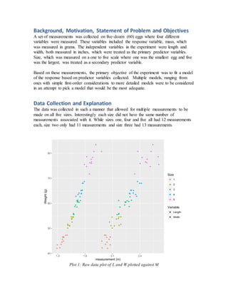
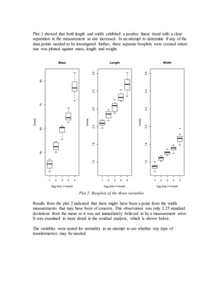
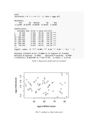
- Measurements were taken of the length, width, size, and mass of 60 eggs to develop a model predicting mass from the other variables. - Initial models using just length and width or adding size did not meet assumptions of constant variance. - The final adequate model included length, width, and a calculated volume variable, meeting assumptions and performing well on cross-validation.

1. Eggs Project
Rochester Institute of Technology
Hans DeSelms and Roopan Verma
February 24, 2016

2. Executive Summary
Measurements were taken on five-dozen eggs in an attempt to fit an adequate model
using primary variables, length and width, as well as a secondary size predictor
variable. Informal plots of the raw data showed a linear positive trend between both
length and width, which also led to the reasonable conclusion that length and width
would be highly correlated with one another.
When creating suitable models, it was quickly realized that a simple model
containing only length and width would not suffice. Through the investigation of
model adequacies and residual analyses, a more complex model was created. The
final model chosen, which met all the residual assumptions and was highly adequate
included length, width, and volume (which was calculated by using length and
width). Results showed a highly adequate model that performed well when a cross-
validation method was applied to check model performance.

3. Background, Motivation, Statement of Problem and Objectives
A set of measurements was collected on five-dozen (60) eggs where four different
variables were measured. These variables included the response variable, mass, which
was measured in grams. The independent variables in the experiment were length and
width, both measured in inches, which were treated as the primary predictor variables.
Size, which was measured on a one to five scale where one was the smallest egg and five
was the largest, was treated as a secondary predictor variable.
Based on these measurements, the primary objective of the experiment was to fit a model
of the response based on predictor variables collected. Multiple models, ranging from
ones with simple first-order considerations to more detailed models were to be considered
in an attempt to pick a model that would be the most adequate.
Data Collection and Explanation
The data was collected in such a manner that allowed for multiple measurements to be
made on all five sizes. Interestingly each size did not have the same number of
measurements associated with it. While sizes one, four and five all had 12 measurements
each, size two only had 11 measurements and size three had 13 measurements.
Plot 1: Raw data plot of L and W plotted against M
40
50
60
70
80
1.5 1.8 2.1 2.4
measurement (in)
Weight(g)
Size
1
2
3
4
5
Variable
Length
Width

4. Plot 1 showed that both length and width exhibited a positive linear trend with a clear
separation in the measurement as size increased. In an attempt to determine if any of the
data points needed to be investigated further, three separate boxplots were created where
size was plotted against mass, length and weight.
Plot 2: Boxplots of the three variables
Results from the plot 2 indicated that there might have been a point from the width
measurements that may have been of concern. This observation was only 2.25 standard
deviations from the mean so it was not immediately believed to be a measurement error.
It was examined in more detail in the residual analysis, which is shown below.
The variables were tested for normality in an attempt to see whether any type of
transformation may be needed.
1 2 3 4 5
50607080
Mass
Egg Size (1=small)
Grams
1 2 3 4 5
1.61.82.02.22.42.6
Length
Egg Size (1=small)
Inches
1 2 3 4 5
1.61.82.02.22.42.6
Width
Egg Size (1=small)
Inches

5. Plot 3: QQ-plots of the variables
In addition to the QQ-plots shown in plot 3, a Shapiro-Wilk test was done on each
variable in order to check for normality.
Shapiro-Wilk normality test
data: eggs.df: Mass
W = 0.958, p-value = 0.0376
Shapiro-Wilk normality test
data: eggs.df: Length
W = 0.96591, p-value = 0.09188
Shapiro-Wilk normality test
-2 -1 0 1 2
50607080
Mass
Theoretical Quantiles
SampleQuantiles
-2 -1 0 1 2
2.02.12.22.32.42.52.6
Length
Theoretical Quantiles
SampleQuantiles
-2 -1 0 1 2
1.51.61.71.81.9
Width
Theoretical Quantiles
SampleQuantiles

6. data: eggs.df: Width
W = 0.98606, p-value = 0.7252
Table 1: Shapiro-Wilk Normality Tests
The results of the Shapiro-Wilk test indicated a low p-value for mass, which meant that
the variable deviated from normality and a transformation may have been needed for
model fitting.
Histograms of the distributions were also created to see if any obvious skew was present
in the data.
Plot 4: Histograms of the raw data
Results showed that length had a bit of a skew, which may be of concern. Nothing was
done with the raw data to correct this but it was something that was noted and would
have been investigated if the model selected had any adequacy problems.
Mass
Egg Size (1=small)
Grams
40 50 60 70 80
051015
Length
Egg Size (1=small)
Inches
2.0 2.2 2.4 2.6
051015
Width
Egg Size (1=small)
Inches
1.5 1.7 1.9
051015

7. Statistical Analysis
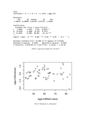
The modeling effort started by constructing the naive regression model of mass as a
linear function of length and width. The summary in table 2 below shows a very high
adjusted r-squared of 0.995. All the p-values were essentially zero as well, indicating that
the intercept and both dependent variables were significant.
Call:
lm(formula = M ~ ., data = eggs.df[, 1:3])
Residuals:
Min 1Q Median 3Q Max
-1.46800 -0.49104 -0.02423 0.43205 2.09134
Coefficients:
Estimate Std. Error t value Pr(>|t|)
(Intercept) -109.775 1.629 -67.38 <2e-16 ***
L 27.354 1.405 19.47 <2e-16 ***
W 63.605 2.046 31.09 <2e-16 ***
---
Signif. codes: 0 '***' 0.001 '**' 0.01 '*' 0.05 '.' 0.1 ' ' 1
Residual standard error: 0.822 on 57 degrees of freedom
Multiple R-squared: 0.9949, Adjusted R-squared: 0.9947
F-statistic: 5566 on 2 and 57 DF, p-value: < 2.2e-16
Shapiro-Wilk normality test
data: eggs.lm$residuals
W = 0.98254, p-value = 0.545
Table 2: naïve regression model
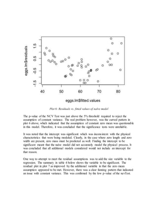
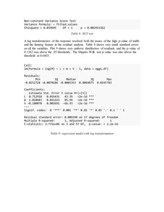
In an attempt to check model adequacy, residual analysis was done on the naïve model by
checking normality, constant variance and non-linearity.

8. Plot 5: QQ-plots of the naïve model
Non-constant Variance Score Test
Variance formula: ~ fitted.values
Chisquare = 3.627081 Df = 1 p = 0.05684644
Table 3: Non-constant variance test
The QQ-Plots of the residuals in plot 5 appeared normal and the high p-value (above
0.05) of the Shapiro-Wilk test reinforced this conclusion.

9. Plot 6: Residuals vs. fitted values of naïve model
The p-value of the NCV Test was just above the 5% threshold required to reject the
assumption of constant variance. The real problem however, was the curved pattern in
plot 6 above, which indicated that the assumption of constant zero mean was questionable
in this model. Therefore, it was concluded that the significance tests were unreliable.
It was noted that the intercept was significant which was inconsistent with the physical
characteristics that were being modeled. Clearly, in the case where zero length and zero
width are present, zero mass must be predicted as well. Finding the intercept to be
significant meant that the naive model did not accurately model the physical process. It
was concluded that all additional models considered would not include an intercept for
that reason.
One way to attempt to meet the residual assumptions was to add the size variable to the
regression. The summary in table 4 below shows the variable to be significant. The
residual plot in plot 7 as improved by the additional variable in that the zero mean
assumption appeared to be met. However, there was a clear fanning pattern that indicated
an issue with constant variance. This was confirmed by the low p-value of the ncvTest.

10. Call:
lm(formula = M ~ L + W + S - 1, data = eggs.df)
Residuals:
Min 1Q Median 3Q Max
-1.12287 -0.42794 0.09545 0.36556 1.29101
Coefficients:
Estimate Std. Error t value Pr(>|t|)
L 25.234 1.525 16.54 <2e-16 ***
W 61.204 2.540 24.10 <2e-16 ***
S1 -101.117 5.497 -18.39 <2e-16 ***
S2 -101.622 5.799 -17.52 <2e-16 ***
S3 -101.396 6.036 -16.80 <2e-16 ***
S4 -101.201 6.259 -16.17 <2e-16 ***
S5 -99.319 6.653 -14.93 <2e-16 ***
---
Signif. codes: 0 '***' 0.001 '**' 0.01 '*' 0.05 '.' 0.1 ' ' 1
Residual standard error: 0.6008 on 53 degrees of freedom
Multiple R-squared: 0.9999, Adjusted R-squared: 0.9999
F-statistic: 8.842e+04 on 7 and 53 DF, p-value: < 2.2e-16
Table 4: Regression model with size included
Plot 7: residual vs. fitted values plot

11. Non-constant Variance Score Test
Variance formula: ~ fitted.values
Chisquare = 9.443896 Df = 1 p = 0.00211853
Table 5: NCV test
The next logical step considered was that the mass of an egg should be closely related to
its volume. A direct measure of volume was not contained in the data set but could be
calculated by using length and width. The equation below represents the formula by
which volume was approximated.
𝑉 = (
2𝜋
3
) (
𝑊
2
)
2𝐿
Modeling mass against the approximation of volume as the sole predictor showed the
predictor was significant with a high r-squared value for the regression based on the
results in table 6 below. However, there were clear problems with the downward sloping
residuals shown in plot 8 below.
Call:
lm(formula = M ~ V - 1, data = eggs.df)
Residuals:
Min 1Q Median 3Q Max
-3.7699 -0.4085 0.3151 0.7490 1.3194
Coefficients:
Estimate Std. Error t value Pr(>|t|)
V 17.32936 0.03314 522.8 <2e-16 ***
---
Signif. codes: 0 '***' 0.001 '**' 0.01 '*' 0.05 '.' 0.1 ' ' 1
Residual standard error: 0.9039 on 59 degrees of freedom
Multiple R-squared: 0.9998, Adjusted R-squared: 0.9998
F-statistic: 2.734e+05 on 1 and 59 DF, p-value: < 2.2e-16
Table 6: regression model of volume as the sole predictor

12. Plot 8: residuals vs. fitted plot
The residuals vs. fitted values plot clearly indicated that the model was not adequate. To
account for this, the original variables, length and width were added back into the model.
It was assumed that there would be a high probability of multicollinearity within the
variables, as all three were highly correlated with one another. However the patterns of
the residuals shown in plot 8 were unacceptable, and needed to be improved.
Multicollinearity can inflate the standard errors of the coefficients causing the rejection of
an otherwise significant coefficient. This may be the reason that the p-value for width
shown in table 7 was so high in the model. The residual pattern was improved in this
model, but it exhibited a fanning feature that was indicative of non-constant variance.
The very low p-value of the NCV Test shown below indicated that the null hypothesis of
constant variance be rejected.

13. Call:
lm(formula = M ~ L + W + V - 1, data = eggs.df)
Residuals:
Min 1Q Median 3Q Max
-2.08255 -0.48909 0.03594 0.41731 1.40762
Coefficients:
Estimate Std. Error t value Pr(>|t|)
L 2.6056 1.1025 2.363 0.0215 *
W -0.4598 1.4200 -0.324 0.7473
V 15.8992 0.1805 88.065 <2e-16 ***
---
Signif. codes: 0 '***' 0.001 '**' 0.01 '*' 0.05 '.' 0.1 ' ' 1
Residual standard error: 0.6306 on 57 degrees of freedom
Multiple R-squared: 0.9999, Adjusted R-squared: 0.9999
F-statistic: 1.872e+05 on 3 and 57 DF, p-value: < 2.2e-16
Table7: regression model of L, W and V
Plot 9: Residuals vs. fitted plots

14. Non-constant Variance Score Test
Variance formula: ~ fitted.values
Chisquare = 8.859695 Df = 1 p = 0.002915362
Table 8: NCV test
A log transformation of the response resolved both the issues of the high p-value of width
and the fanning feature in the residual analysis. Table 8 shows very small standard errors
on all the variables. Plot 9 shows very uniform distribution of residuals and the p-value of
0.1362 was above the .05 thresholds. The Shapiro-Wilk test p-value was also above the
threshold at 0.6403.
Call:
lm(formula = log(M) ~ L + W + V - 1, data = eggs.df)
Residuals:
Min 1Q Median 3Q Max
-0.0252728 -0.0070186 -0.0005353 0.0069875 0.0195783
Coefficients:
Estimate Std. Error t value Pr(>|t|)
L 0.712918 0.016431 43.39 <2e-16 ***
W 1.818683 0.021163 85.94 <2e-16 ***
V -0.180078 0.002691 -66.93 <2e-16 ***
---
Signif. codes: 0 '***' 0.001 '**' 0.01 '*' 0.05 '.' 0.1 ' ' 1
Residual standard error: 0.009398 on 57 degrees of freedom
Multiple R-squared: 1, Adjusted R-squared: 1
F-statistic: 3.771e+06 on 3 and 57 DF, p-value: < 2.2e-16
Table 8: regression model with log transformation

15. Plot 10: Residuals vs. fitted values plot
Plot 11: Residual Analysis of regression model

16. The residual graphs in plot 11 above indicated that observation 17 warranted further
investigation due to its relatively high leverage point and with its Cook's Distance value
which was greater than one. The values of this observation were:
M L W S LW V
17 80.7 2.377 1.979 5 4.704083 4.87438
This was a slightly unusual egg in that its 1.98-inch width measurement was the
maximum in the data set, but its 2.38-inch length only ranked just above the 3rd quartile.
Its mass was very near the top of the range at 80.7 grams. That might have led to the
conclusion that the length was measured incorrectly low, but its calculated volume of
4.87 cubic inches was also at the very high end of the range so there was no reason to
suspect a measurement error. This egg was just a little rounder than the others that were
measured. Based on this, the observation was retained in the analysis. Observations with
high Cook's Distances are not always bad. They simply have more effect of the value of
the model parameters than other observations.
The final step in the modeling process was to evaluate the model performance and
variance through cross-validation. Table 9 below shows very robust results from a 10-
fold cross-validation repeated 10 times. The root mean squared error was below 1% with
a 0.33% standard deviation and R-squared is nearly 99.8% with only a 0.15% standard
deviation.
Linear Regression
60 samples
5 predictor
No pre-processing
Resampling: Cross-Validated (10 fold, repeated 10 times)
Summary of sample sizes: 53, 54, 56, 55, 54, 54, ...
Resampling results
RMSE Rsquared RMSE SD Rsquared SD
0.009799897 0.9980778 0.003119053 0.001284406
Table 9: Cross Validation results
Evaluation of Results
Many steps were taken to ensure the best possible model was created for this experiment.
Many considerations were taken into account in an attempt to have the most adequate
model. This included investigating higher order terms as well as the effect that size had
on mass along with the primary predictor variables of length and width.

17. The final model that was selected included a model with significant variables length,
width and volume. The model proved to be extremely adequate as shown by the high r-
squared values and the fact that all residual assumptions were met. The model’s adequacy
was further proved by robust results obtained through cross-validation.
By looking at the raw data plots during the informal analysis phase, it was theorized that
length and width as well as size would be needed to fit the most adequate model. This
was due to the clear separation presented in plot 1. The final selected model revealed that
although length and width were necessary, size had no impact on model adequacy and
was discarded. Plot 3 and table 1 also indicated that the response would need to be
transformed as it failed the Shapiro-Wilk test and that too was confirmed in the final
model. The r-squared value of one and the extremely low p-values of the predictors
allowed for the conclusion that this was in-fact the best model that could be fit for this
data-set.

18. Appendix – R Code
library(car)
library(forecast)
library(glmnet)
eggs.df<-read.table("Eggs.txt",header = TRUE, sep = "t")
str(eggs.df)
eggs.df$S<-as.factor(eggs.df$S)
summary(scale(eggs.df[which(eggs.df$S==5),1:3]))
cor(eggs.df[,1:3])
## Question 1
units<-c("Grams","Inches","Inches")
titles<-c("Mass", "Length", "Width")
quartz()
par(mfrow=c(1,3))
boxplot(eggs.df[,1]~eggs.df$S, main=titles[1],
xlab="Egg Size (1=small)",ylab=units[1])
for (i in 2:3){
boxplot(eggs.df[,i]~eggs.df$S, main=titles[i],
ylim=c(min(eggs.df[,2:3]),max(eggs.df[,2:3])),
xlab="Egg Size (1=small)",ylab=units[i])
}
## or
quartz()
par(mfrow=c(1,3))
for (i in 1:3){
boxplot(eggs.df[,i]~eggs.df$S, main=titles[i],
xlab="Egg Size (1=small)",ylab=units[i])
}

19. ## Histograms
quartz()
par(mfrow=c(1,3))
for (i in 1:3){
hist(eggs.df[,i], main=titles[i], ylim = c(0,15),
xlab="Egg Size (1=small)",ylab=units[i])
# lines(density(eggs.df[,i]), col="blue", lwd=2)
}
# Notice Skew of Length
## Check Normality
quartz()
par(mfrow=c(1,3))
for (i in 1:3){
qqnorm(eggs.df[,i],main=titles[i])
qqline(eggs.df[,i])
}
shapiro.test(eggs.df[,1])
shapiro.test(eggs.df[,2])
shapiro.test(eggs.df[,3])
# Appears Normal
## Question 2.d without S
eggs.lm<-lm(M~., data=eggs.df[,1:3])
summary(eggs.lm)

20. quartz()
plot(eggs.lm$fitted.values, eggs.lm$residuals)
## clear pattern to residuals.
residualPlots(eggs.lm)
## curved lines show non constant mean
shapiro.test(eggs.lm$residuals)
quartz()
qqnorm(eggs.lm$residuals,main="Naive LM Residual QQ-Plot")
qqline(eggs.lm$residuals)
## QQ-Plots of residuals above appear normal
ncvTest(eggs.lm)
accuracy(eggs.lm)
## Question 2.e with S
eggs.lm<-lm(M~., data=eggs.df)
summary(eggs.lm)
quartz()
plot(eggs.lm$fitted.values, eggs.lm$residuals)
## no pattern to residuals.
residualPlots(eggs.lm, main="Residual Plots with Size Variable")
## straight lines show constant mean
shapiro.test(eggs.lm$residuals)

21. quartz()
qqnorm(eggs.lm$residuals,main="Naive LM Residual QQ-Plot")
qqline(eggs.lm$residuals)
## appear normal
ncvTest(eggs.lm)
accuracy(eggs.lm)