Copyright ©2015 Pearson Education, Inc.6-Chapter 6.docx

Copyright ©2015 Pearson Education, Inc.
6-*
Chapter
6
6-*
Chapter
6
Continuous Probability Distributions
CHAPTER 6 MAP
6.1 Continuous Random Variables
6.2 Normal Probability Distributions
6.3 Exponential Probability Distributions
6.4 Uniform Probability Distributions
6-*

Probability Distributions
Discrete
Ch. 5
Ch. 6
6-*
6.1 Continuous Random Variables
Continuous random variables are outcomes that take on any
numerical value in an interval, as determined by conducting an
experimentUsually measured rather than countedExamples of
continuous data include time, distance, and weight
The purpose of this chapter is to identify the probability that a
specified range of values will occur for continuous random
variables, using continuous probability distributions
6-*
Continuous Random Variables
Continuous random variables can take on any value within a
specified interval
Because there are an infinite number of possible values, the
probability of one specific value occurring is theoretically equal
to zero
Probabilities are based on intervals, not individual
valuesProbability is represented by an area under the
probability distribution

6-*
The remaining sections in chapter 6 address specific continuous
probability distributions
Normal
Uniform
Exponential
Specific Continuous
Section 6.2
Section 6.3
Section 6.4
6-*
Continuous probability distributions can have a variety of
shapes
Shapes of the three common continuous distributions to be
discussed in this chapter:
6-*
The normal probability distribution is useful when the data tend
to fall into the center of the distribution and when very high and
very low values are fairly rare
The exponential distribution is used to describe data where
lower values tend to dominate and higher values don’t occur

very often
The uniform distribution describes data where all the values
have the same chance of occurring
Normal
Uniform
Exponential
6-*
6.2 Normal Probability Distributions
Normal
Uniform
Exponential
Specific Continuous
6-*
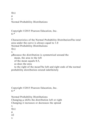
Characteristics of the Normal Probability DistributionThe
distribution is bell-shaped and symmetrical around the
meanBecause the shape of the
distribution is symmetrical,
the mean and median
are the same valueValues near the mean, where
the curve is the tallest, have
a higher likelihood of occurring
than values far from the mean,
where the curve is shorter
Mean
= Median
x

f(x)
μ
σ
Normal Probability Distributions
6-*
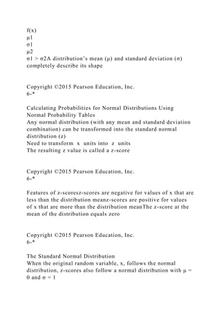
Characteristics of the Normal Probability DistributionThe total
area under the curve is always equal to 1.0
f(x)
x
μBecause the distribution is symmetrical around the
mean, the area to the left
of the mean equals 0.5,
as does the area
to the right of the meanThe left and right ends of the normal
probability distribution extend indefinitely
6-*
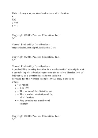
Changing μ shifts the distribution left or right
Changing σ increases or decreases the spread
x
f(x)
μ
σ2
x

f(x)
μ1
σ1
μ2
σ1 > σ2A distribution’s mean (μ) and standard deviation (σ)
completely describe its shape
6-*
Calculating Probabilities for Normal Distributions Using
Normal Probability Tables
Any normal distribution (with any mean and standard deviation
combination) can be transformed into the standard normal
distribution (z)
Need to transform x units into z units
The resulting z value is called a z-score
6-*
Features of z-scoresz-scores are negative for values of x that are
less than the distribution meanz-scores are positive for values
of x that are more than the distribution meanThe z-score at the
mean of the distribution equals zero
6-*
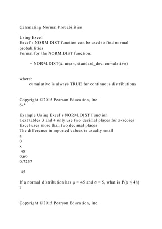
The Standard Normal Distribution
When the original random variable, x, follows the normal
distribution, z-scores also follow a normal distribution with μ =
0 and σ = 1

This is known as the standard normal distribution
x
f(x)
μ = 0
σ = 1
6-*
https://istats.shinyapps.io/NormalDist/
6-*
A probability density function is a mathematical description of
a probability distributionrepresents the relative distribution of
frequency of a continuous random variable
Formula for the Normal Probability Density Function:
where:
e = 2.71828
π = 3.14159
μ = The mean of the distribution
σ = The standard deviation of the
distribution
x = Any continuous number of
interest
6-*

Calculating Normal Probabilities
Using Excel
Excel’s NORM.DIST function can be used to find normal
probabilities
Format for the NORM.DIST function:
= NORM.DIST(x, mean, standard_dev, cumulative)
where:
cumulative is always TRUE for continuous distributions
6-*
Example Using Excel’s NORM.DIST Function
Text tables 3 and 4 only use two decimal places for z-scores
Excel uses more than two decimal places
The difference in reported values is usually small
z
0
x
48
0.60
0.7257
45
If a normal distribution has μ = 45 and σ = 5, what is P(x ≤ 48)
?

6-*
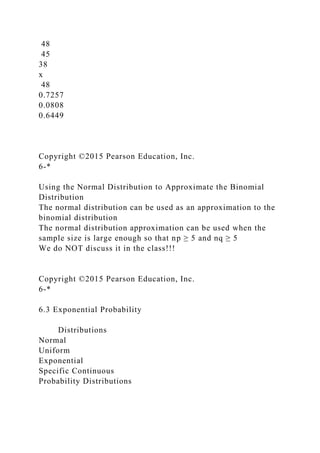
Other Normal Probability Intervals
Example: Probability between two values
Suppose income is normally distributed for a group of workers,
with μ = $45,000 and σ = $5,000
Find the probability that a randomly selected worker from this
group has an income between $38,000 and $48,000
(Can convert all values to
1000s to simplify)
z
0
Probability = ?
45
38
x
48
6-*
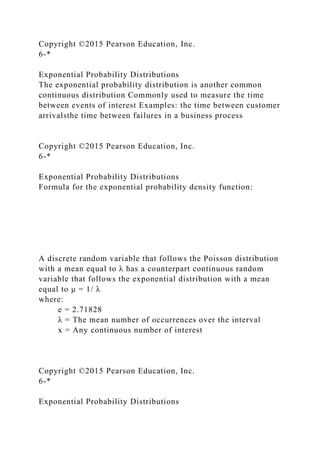
Other Normal Probability Intervals
Example: (continued)
45
38
x
48
45
38
x

48
45
38
x
48
0.7257
0.0808
0.6449
6-*
Using the Normal Distribution to Approximate the Binomial
Distribution
The normal distribution can be used as an approximation to the
binomial distribution
The normal distribution approximation can be used when the
sample size is large enough so that np ≥ 5 and nq ≥ 5
We do NOT discuss it in the class!!!
6-*
6.3 Exponential Probability
Distributions
Normal
Uniform
Exponential
Specific Continuous

6-*
Exponential Probability Distributions
The exponential probability distribution is another common
continuous distribution Commonly used to measure the time
between events of interest Examples: the time between customer
arrivalsthe time between failures in a business process
6-*
Formula for the exponential probability density function:
A discrete random variable that follows the Poisson distribution
with a mean equal to λ has a counterpart continuous random
variable that follows the exponential distribution with a mean
equal to μ = 1/ λ
where:
e = 2.71828
λ = The mean number of occurrences over the interval
x = Any continuous number of interest
6-*

The shape of the exponential distribution depends on the value λ
f(x)
x
λ = 2.0
(mean = 0.5)
λ = 1.0
(mean = 1.0)
λ = 3.0
(mean = .333)
Compared to normal distributions:The exponential distribution
is right-skewed, not symmetricalThe shape is completely
described by only one parameter, λThe values for an
exponential random variable cannot be negative
6-*
Formula for the Exponential Cumulative Distribution Function
where:
e = 2.71828
λ = The mean number of occurrences over the interval
a = Any number of interest
6-*
Calculating Exponential Probabilities Using Excel
Excel’s EXPON.DIST function can be used to find exponential
probabilities
Format for the EXPON.DIST function:

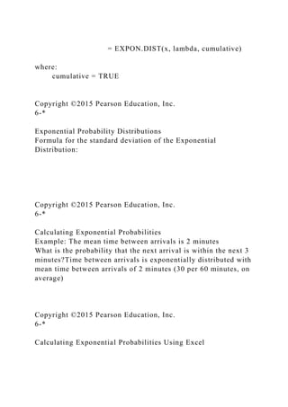
= EXPON.DIST(x, lambda, cumulative)
where:
cumulative = TRUE
6-*
Formula for the standard deviation of the Exponential
Distribution:
6-*
Calculating Exponential Probabilities
Example: The mean time between arrivals is 2 minutes
What is the probability that the next arrival is within the next 3
minutes?Time between arrivals is exponentially distributed with
mean time between arrivals of 2 minutes (30 per 60 minutes, on
average)
6-*
Calculating Exponential Probabilities Using Excel

6-*
6.4 Uniform Probability Distributions
Normal
Uniform
Exponential
Specific Continuous
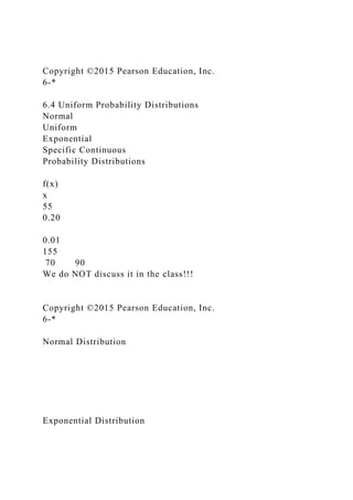
f(x)
x
55
0.20
0.01
155
70 90
We do NOT discuss it in the class!!!
6-*
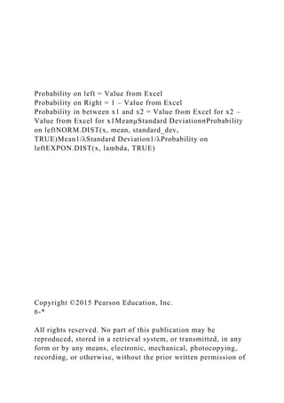
Normal Distribution
Exponential Distribution

Probability on left = Value from Excel
Probability on Right = 1 – Value from Excel
Probability in between x1 and x2 = Value from Excel for x2 –
Value from Excel for x1MeanµStandard DeviationσProbability
on leftNORM.DIST(x, mean, standard_dev,
TRUE)Mean1/λStandard Deviation1/λProbability on
leftEXPON.DIST(x, lambda, TRUE)
6-*
All rights reserved. No part of this publication may be
reproduced, stored in a retrieval system, or transmitted, in any
form or by any means, electronic, mechanical, photocopying,
recording, or otherwise, without the prior written permission of

the publisher.
Printed in the United States of America.
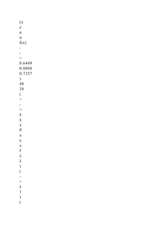
0.5
=
<
<
¥
-
μ)
x
P(
0.5
=
¥
<
<
)
x
P(
μ
1.0
=
¥
<
<
¥
-
)
x
P(
2
2
1
]
(1/2)[
μ)/σ

(x
e
π
σ
f(x)
-
-
=
0.6449
0.0808
0.7257
)
48
38
(
=
-
=
£
£
x
P
x
e
x
f
λ
λ
)
(
-
=
λ
1
)
(

a
e
a
x
P
-
-
=
£
λ
1
=
=
m
s

Copyright ©2015 Pearson Education, Inc.6-Chapter 6.docx

More Related Content

Similar to Copyright ©2015 Pearson Education, Inc.6-Chapter 6.docx

More from bobbywlane695641

Recently uploaded

Copyright ©2015 Pearson Education, Inc.6-Chapter 6.docx