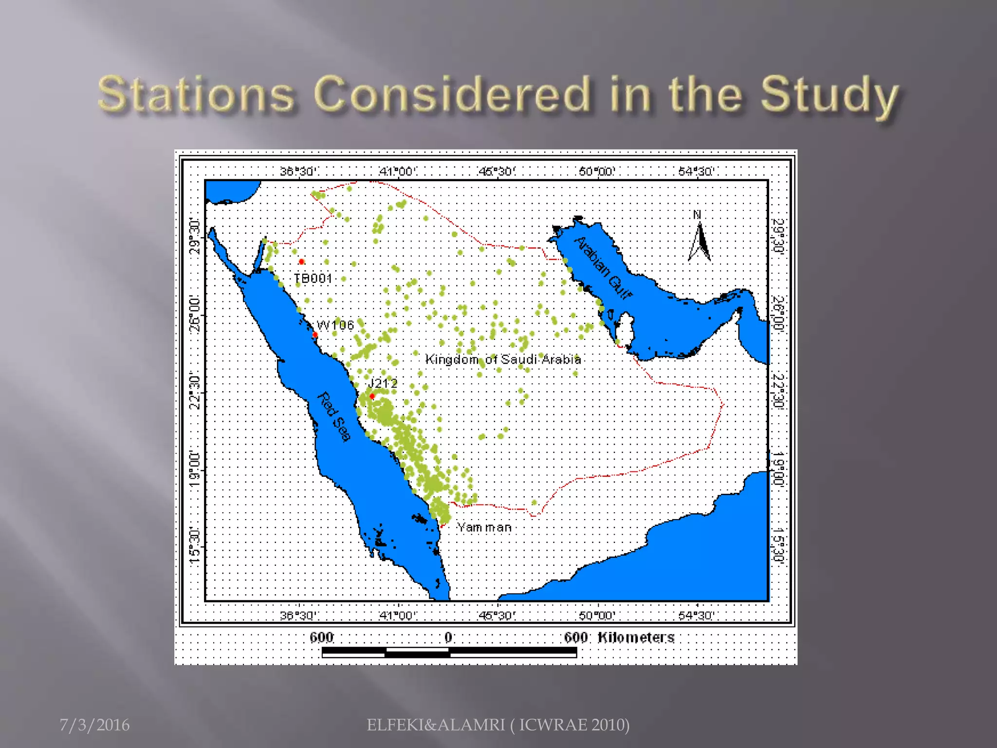
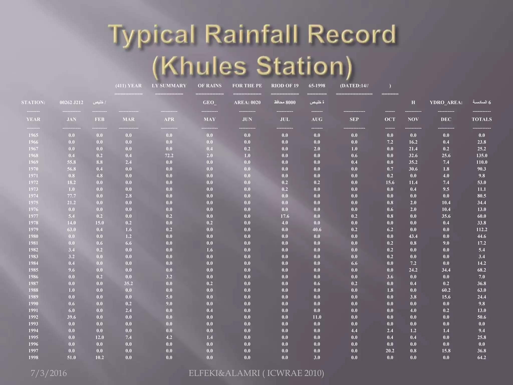
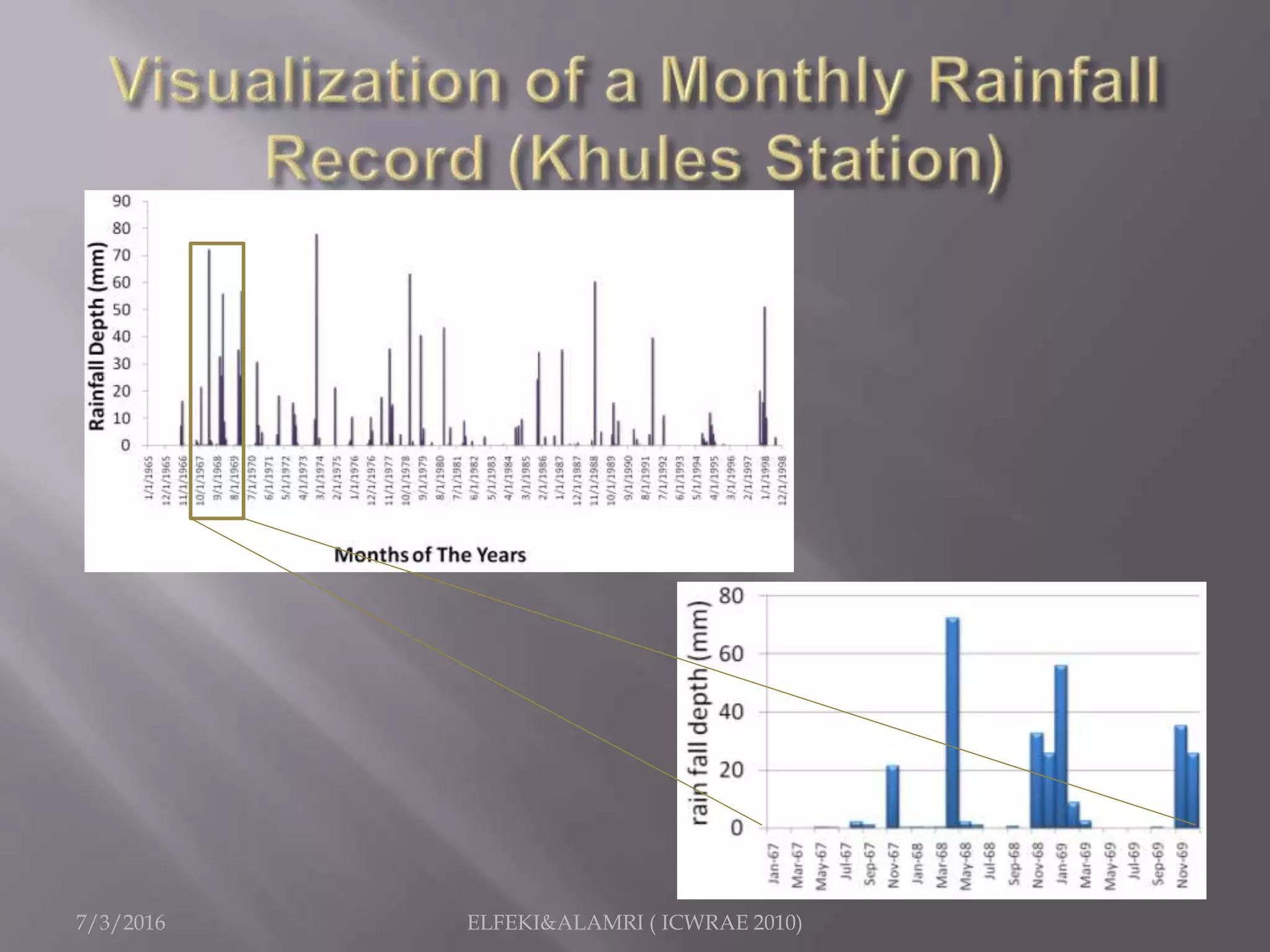
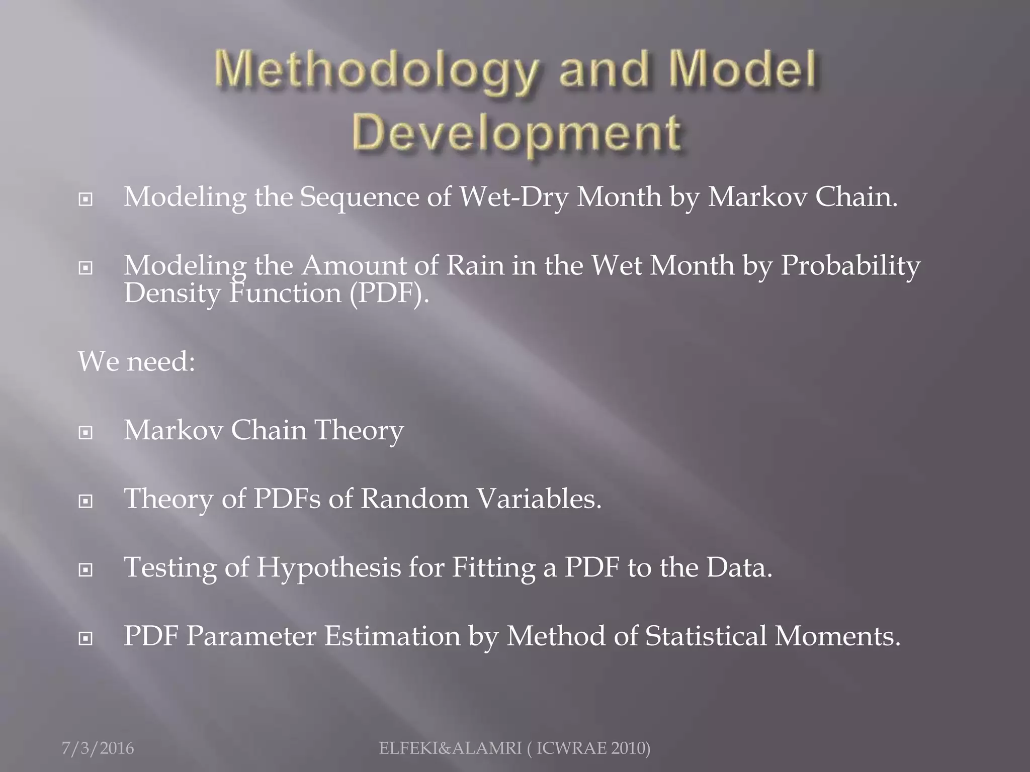
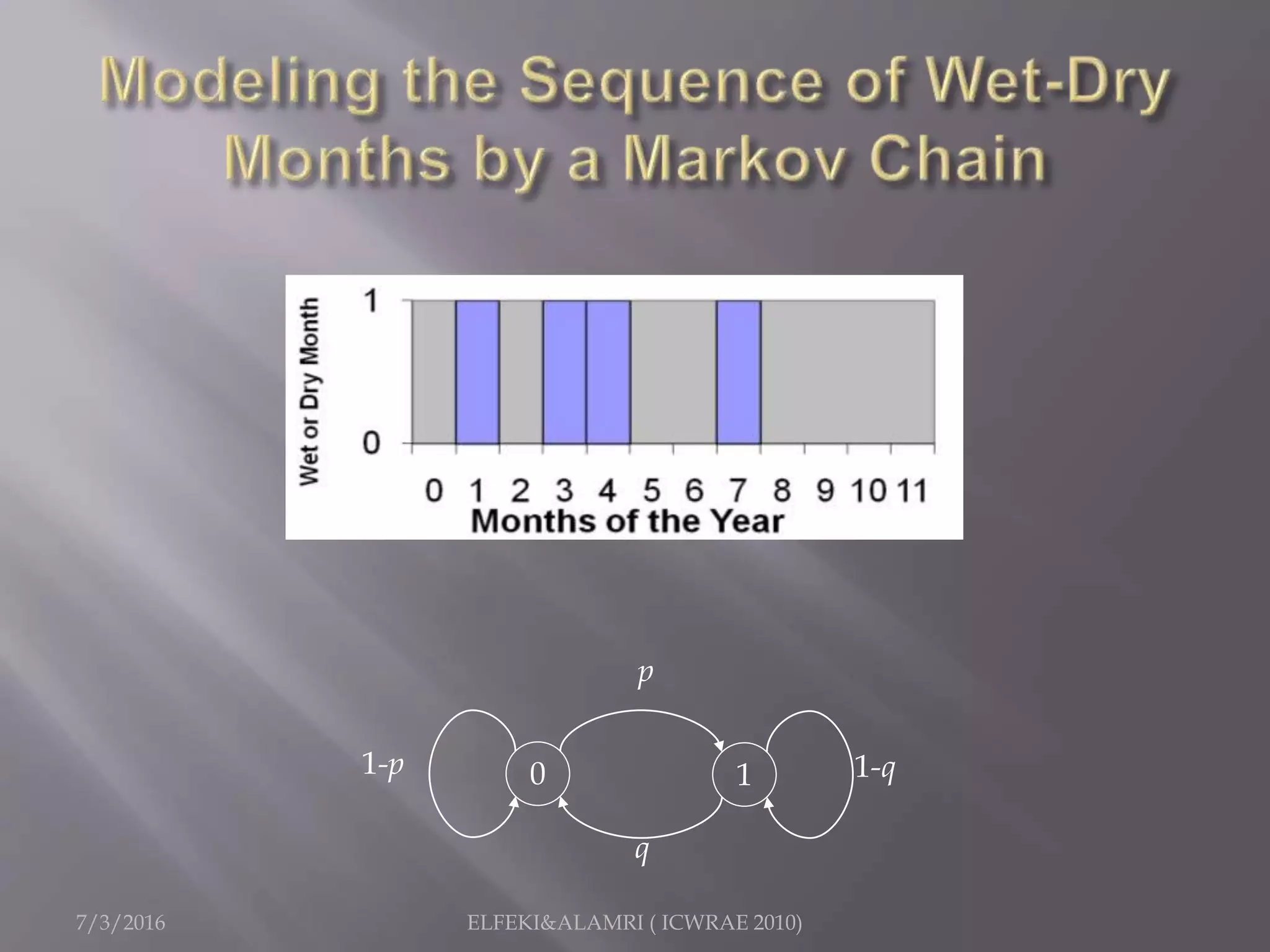
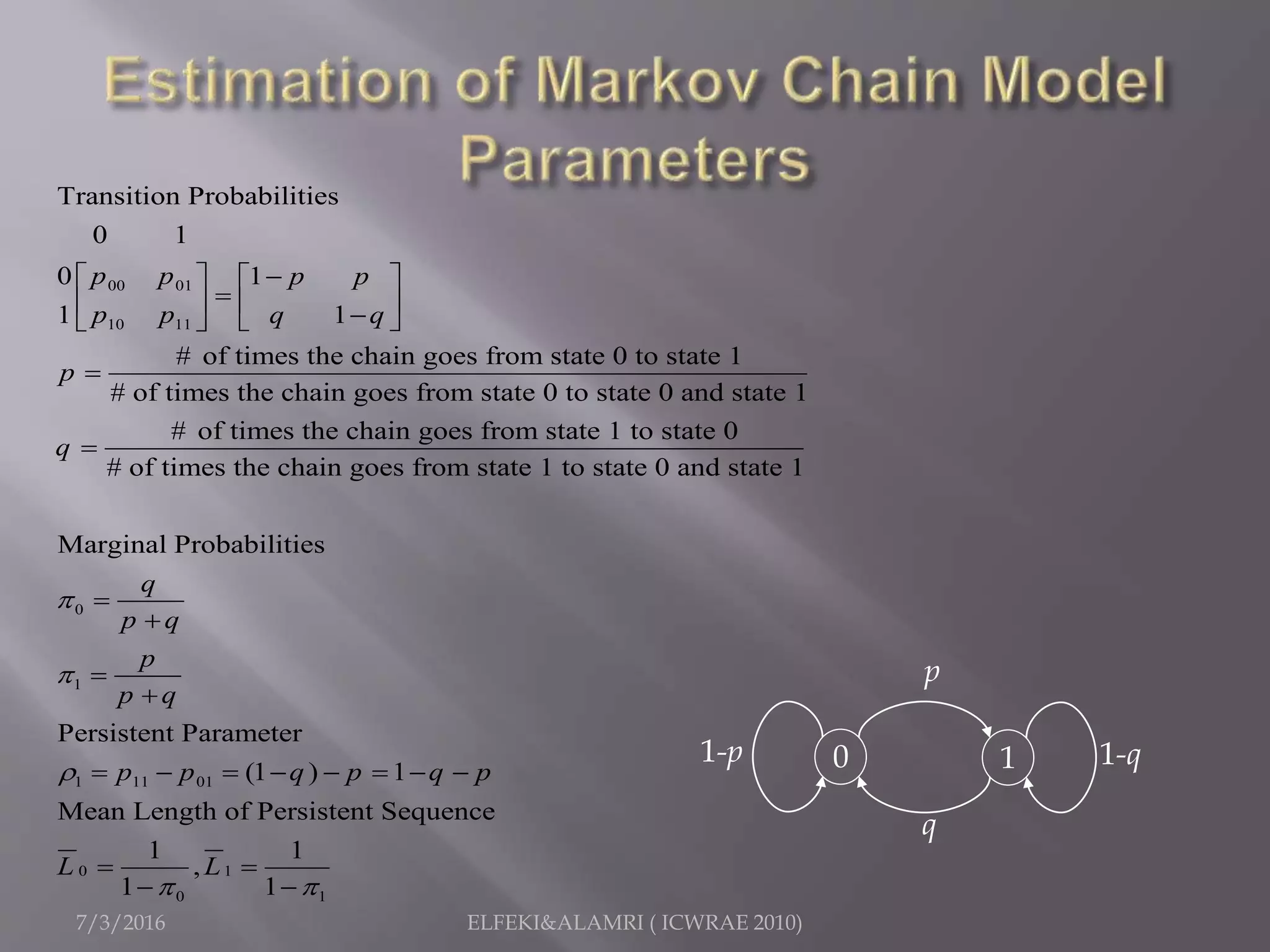
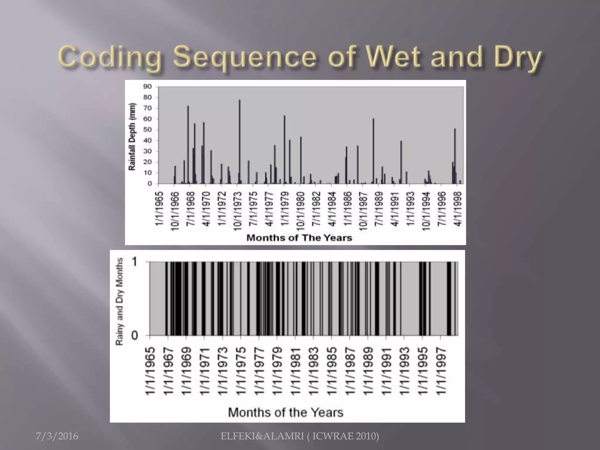
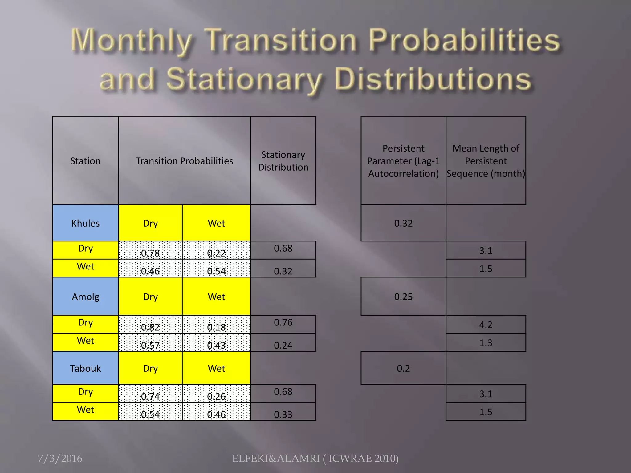
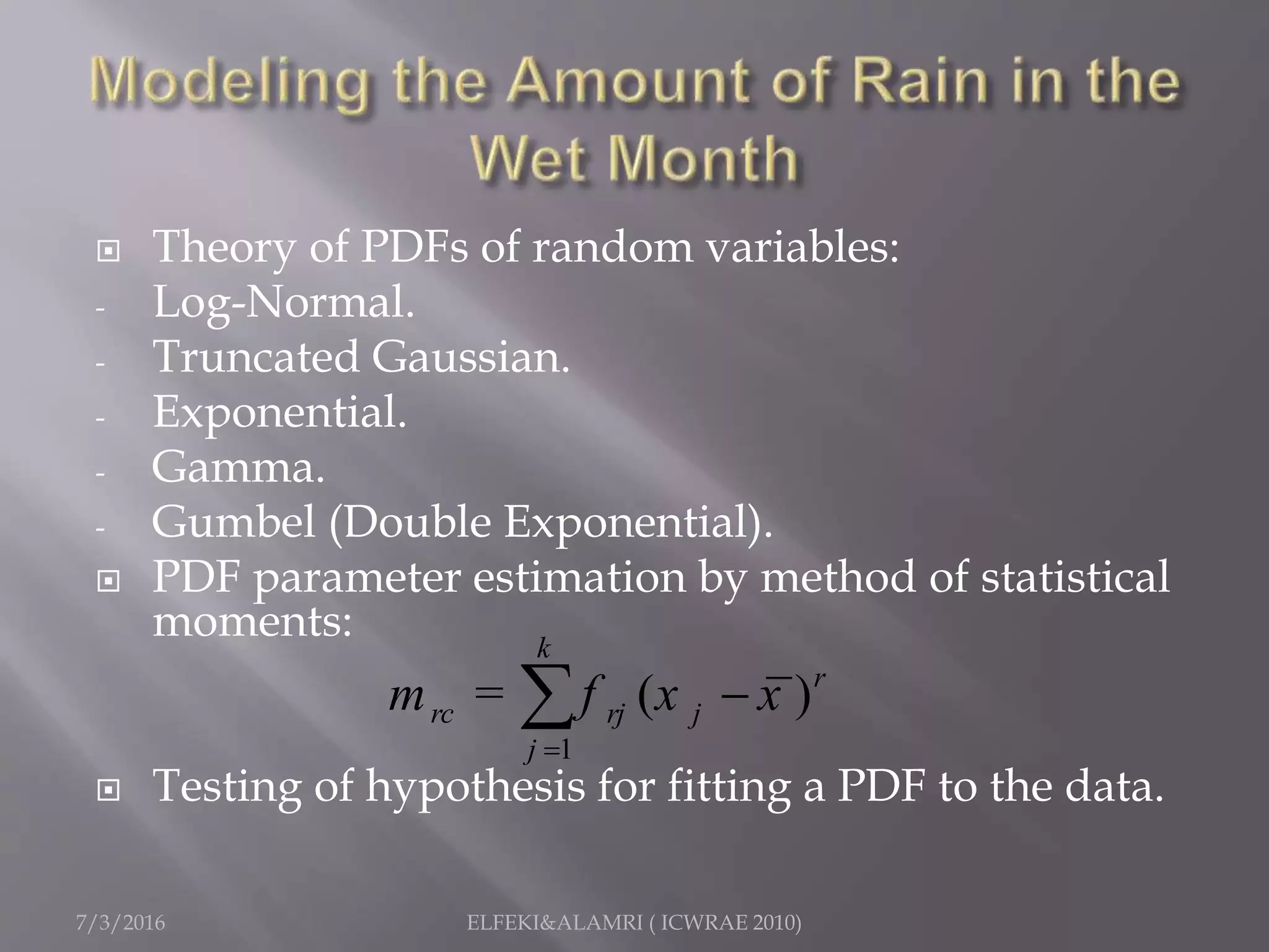
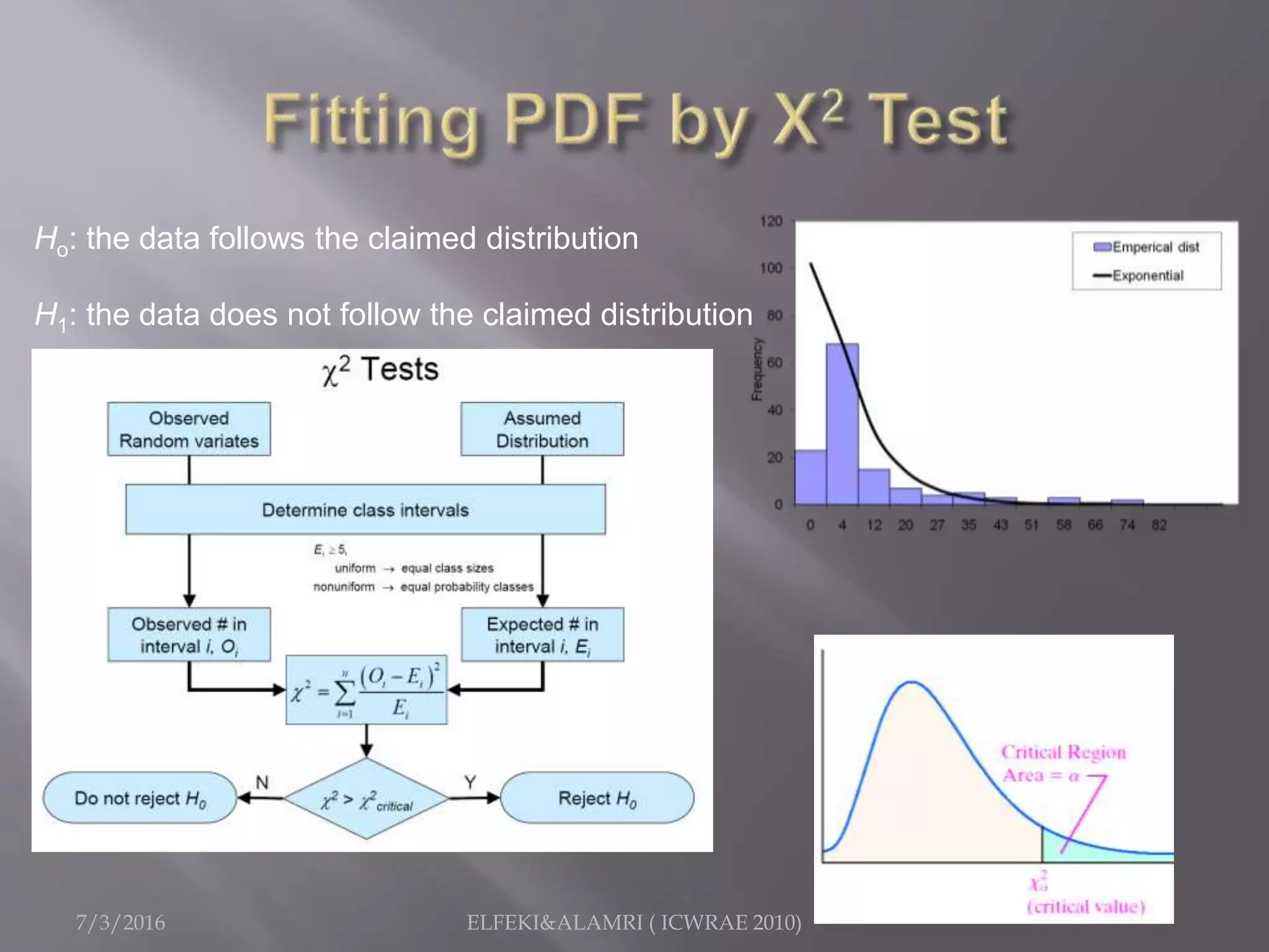
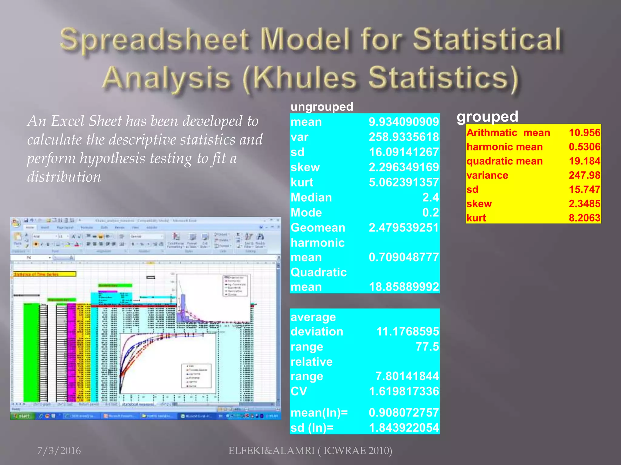
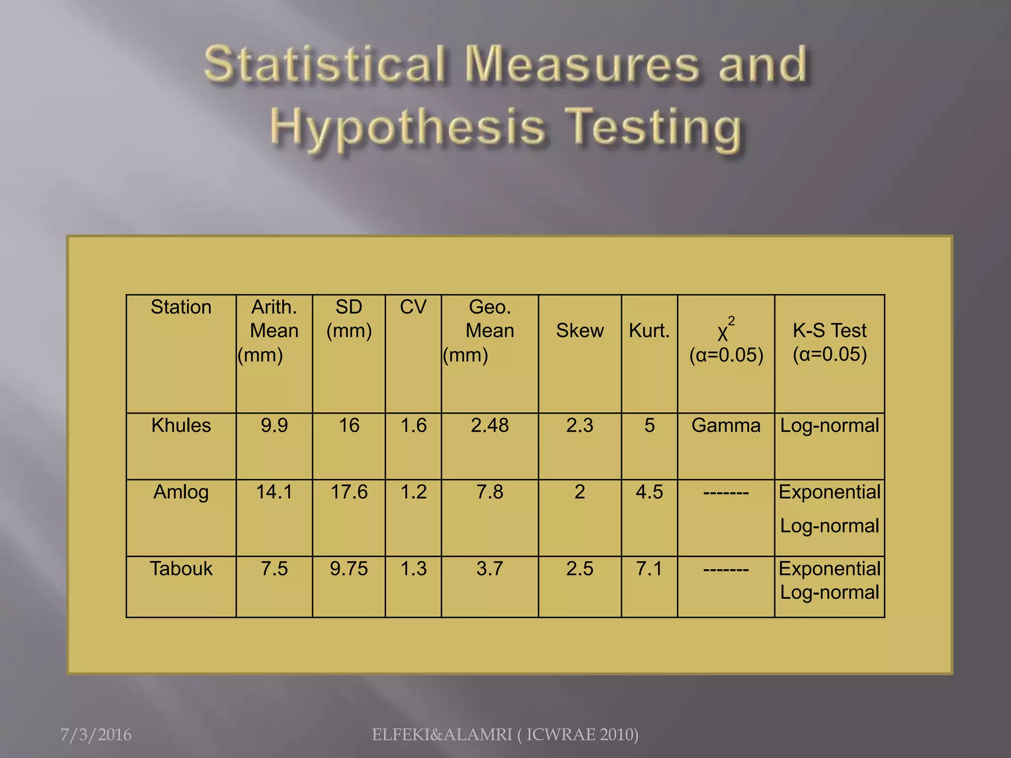
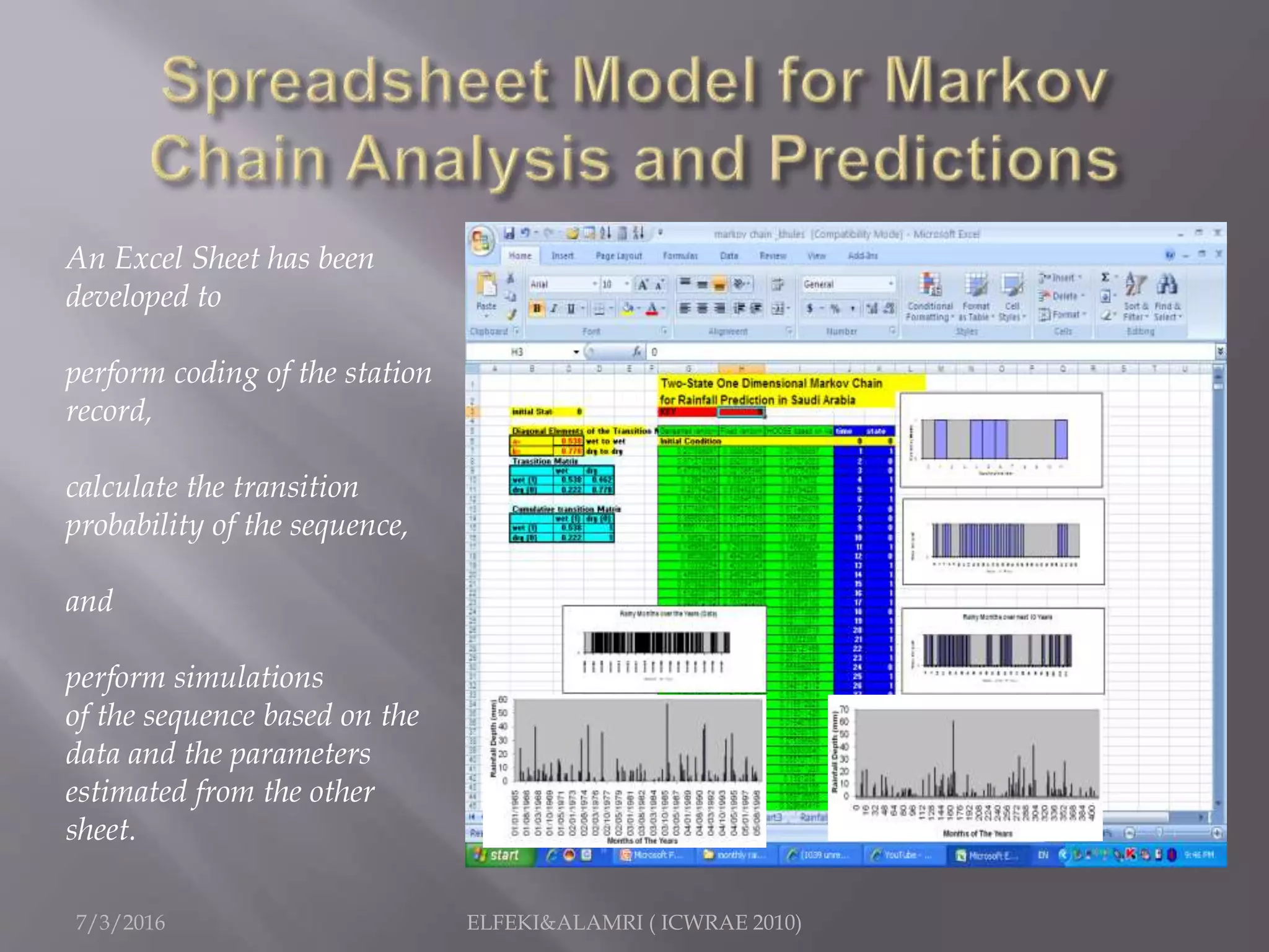
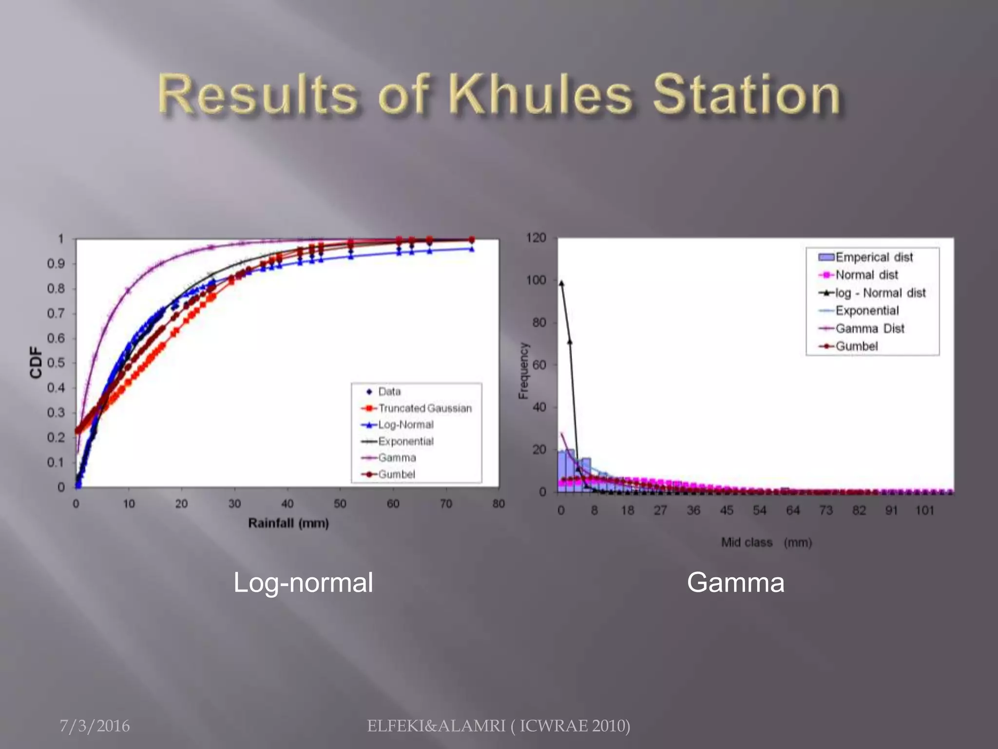
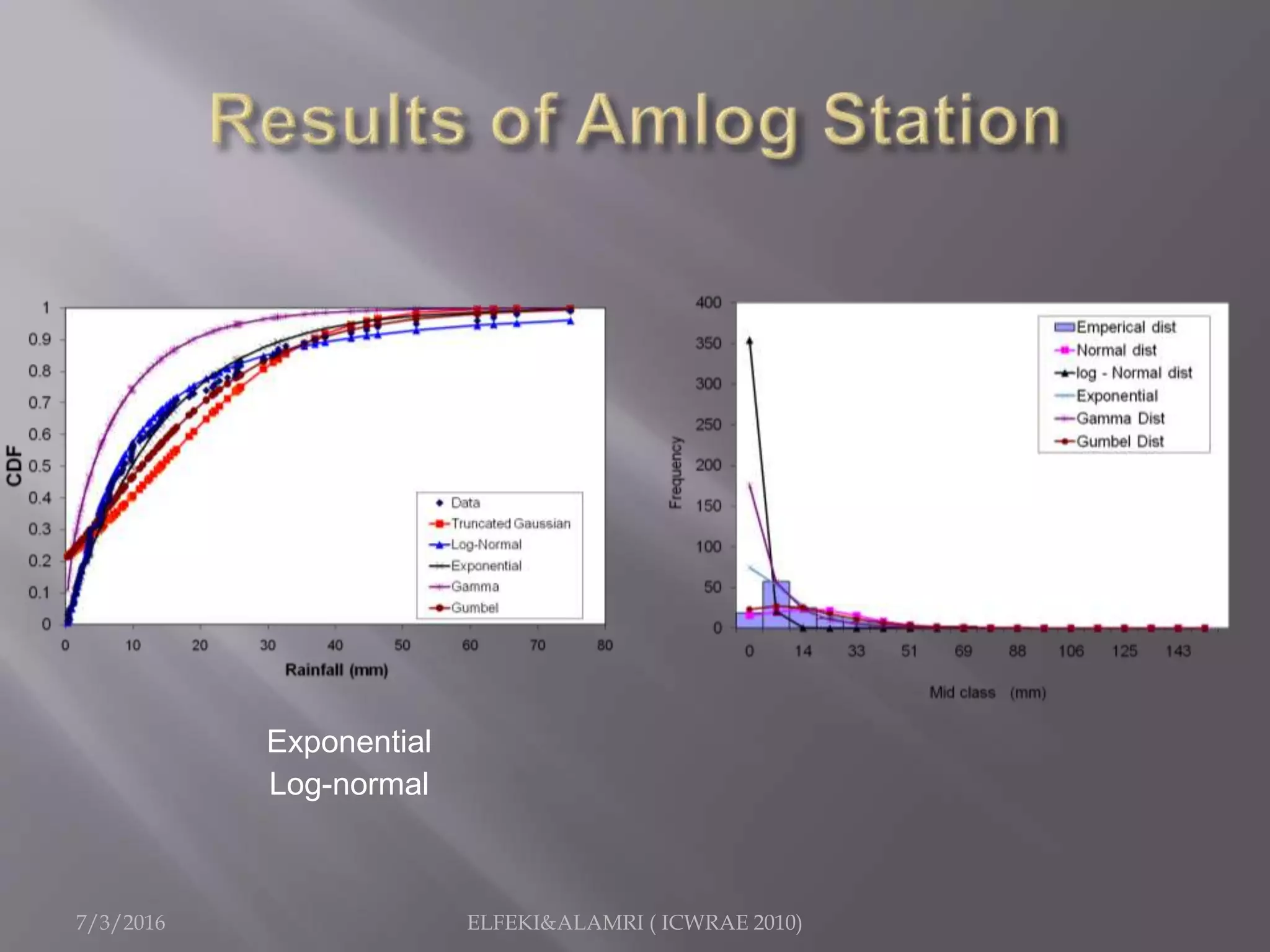
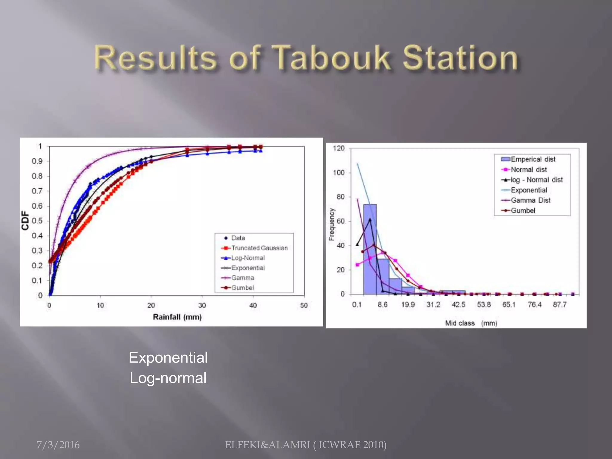
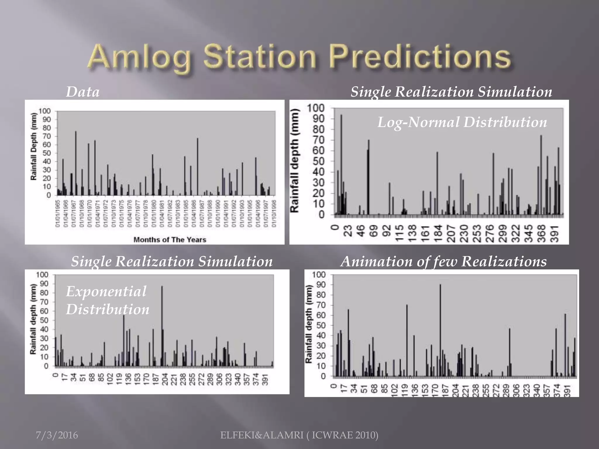
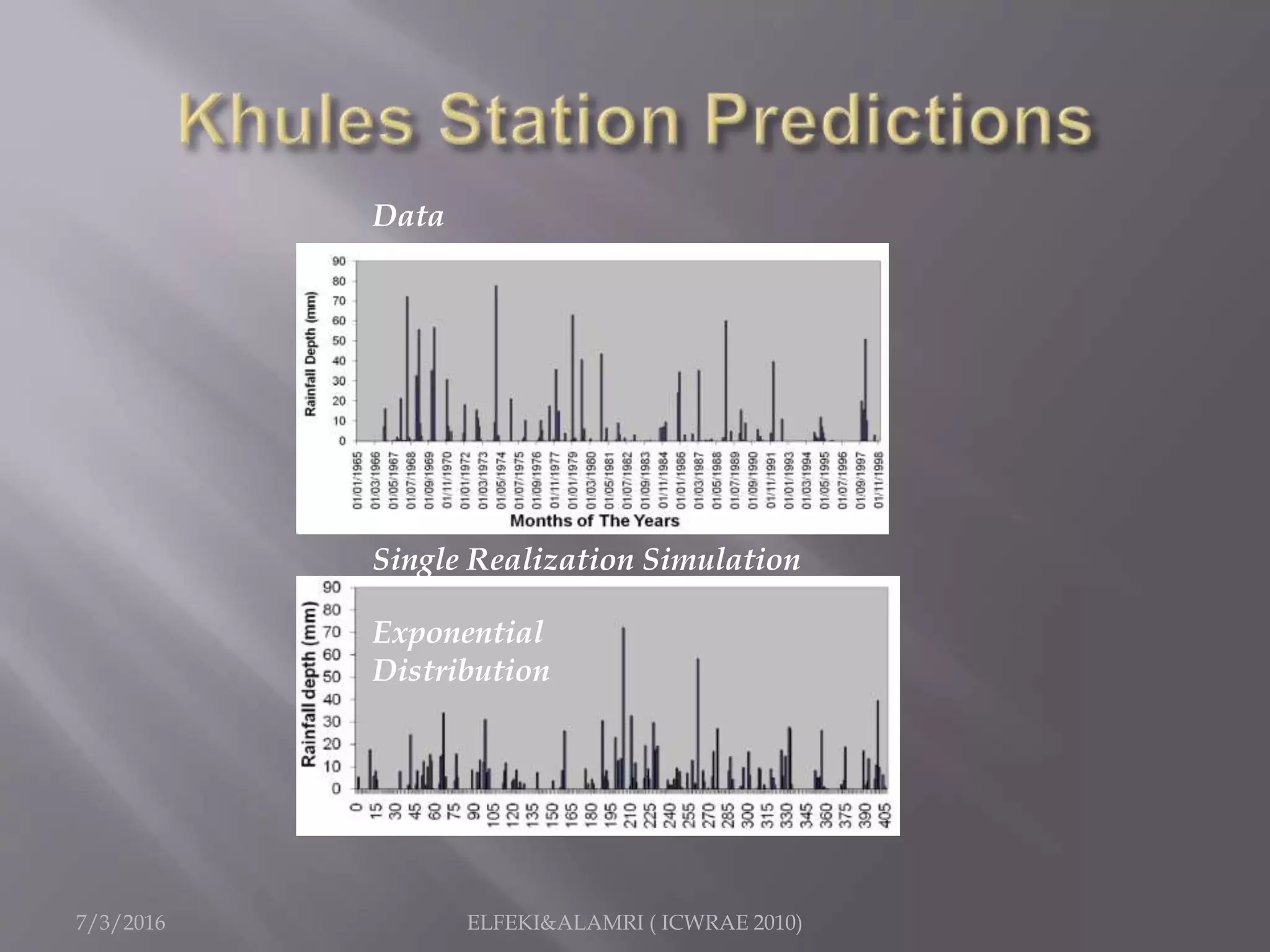
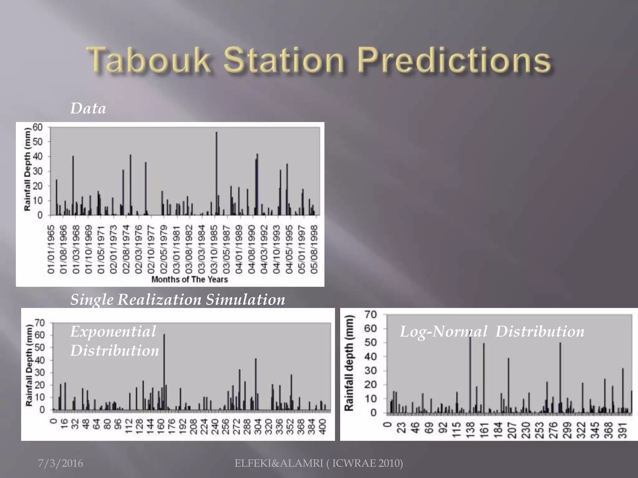
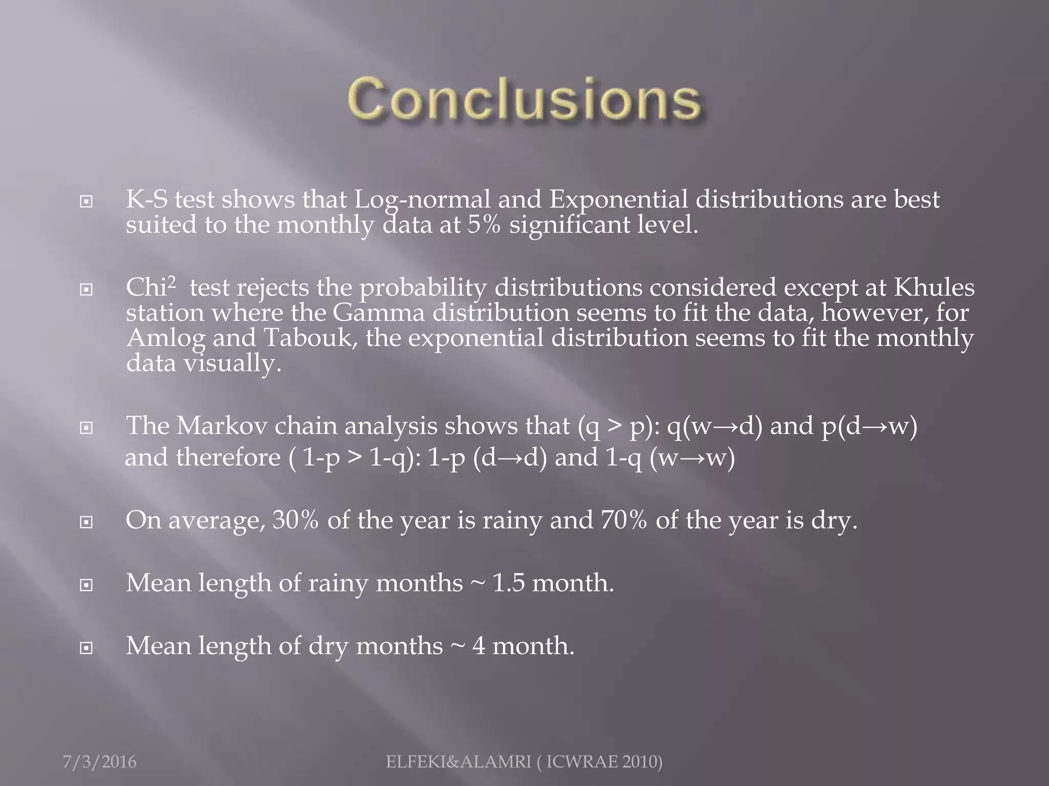
7/3/2016 ELFEKI&ALAMRI ( ICWRAE 2010)
Amro Elfeki and Nassir Al-Amri
Dept. of Hydrology and Water Resources Management ,Faculty of
Meteorology, Environment & Arid Land Agriculture, King Abdulaziz
University , P.O. Box 80208 Jeddah 21589 Saudi Arabia
 Research Objectives
 Typical Rainfall Station Data
 Methodology and Model Development
 Results
 Conclusions
 Outlook
7/3/2016 ELFEKI&ALAMRI ( ICWRAE 2010)
 Modeling monthly rainfall records in arid
zones for future predictions of monthly
rainfall.
 Application on a case study in Saudi Arabia
(Three Stations).
7/3/2016 ELFEKI&ALAMRI ( ICWRAE 2010)
(411) YEAR LY SUMMARY OF RAINS FOR THE PE RIOD OF 19 65-1998 (DATED:14// )
========== ========== ========== ========== ========== ======= ============= ======
STATION: 00262 J212 /‫خليص‬ GEO_ AREA: 0020 8000‫محافظ‬ ‫خليـص‬ ‫ة‬ H YDRO_AREA: 6‫السادسـة‬
-------- ----------- --------- ------------ ---------- ---------- ---------- ---------- ------- ------------- ------ ---------- ---------- -----------
YEAR JAN FEB MAR APR MAY JUN JUL AUG SEP OCT NOV DEC TOTALS
-------- ----------- --------- ------------ ---------- ---------- ---------- ---------- ------- ------------- ------ ---------- ---------- -----------
1965 0.0 0.0 0.0 0.0 0.0 0.0 0.0 0.0 0.0 0.0 0.0 0.0 0.0
1966 0.0 0.0 0.0 0.0 0.0 0.0 0.0 0.0 0.0 7.2 16.2 0.4 23.8
1967 0.0 0.0 0.0 0.0 0.4 0.2 0.0 2.0 1.0 0.0 21.4 0.2 25.2
1968 0.4 0.2 0.4 72.2 2.0 1.0 0.0 0.0 0.6 0.0 32.6 25.6 135.0
1969 55.8 8.8 2.4 0.0 0.0 0.0 0.0 0.0 0.4 0.0 35.2 7.4 110.0
1970 56.8 0.4 0.0 0.0 0.0 0.0 0.0 0.0 0.0 0.7 30.6 1.8 90.3
1971 0.8 4.8 0.0 0.0 0.0 0.0 0.0 0.0 0.0 0.2 0.0 4.0 9.8
1972 18.2 0.0 0.0 0.0 0.0 0.0 0.2 0.2 0.0 15.6 11.4 7.4 53.0
1973 1.0 0.0 0.0 0.0 0.0 0.0 0.2 0.0 0.0 0.0 0.4 9.5 11.1
1974 77.7 0.0 2.8 0.0 0.0 0.0 0.0 0.0 0.0 0.0 0.0 0.0 80.5
1975 21.2 0.0 0.0 0.0 0.0 0.0 0.0 0.0 0.0 0.8 2.0 10.4 34.4
1976 0.0 0.0 0.0 0.0 0.0 0.0 0.0 0.0 0.0 0.6 2.0 10.4 13.0
1977 5.4 0.2 0.0 0.2 0.0 0.0 17.6 0.0 0.2 0.8 0.0 35.6 60.0
1978 14.0 15.0 0.2 0.0 0.2 0.0 4.0 0.0 0.0 0.0 0.0 0.4 33.8
1979 63.0 0.4 1.6 0.2 0.0 0.0 0.0 40.6 0.2 6.2 0.0 0.0 112.2
1980 0.0 0.0 1.2 0.0 0.0 0.0 0.0 0.0 0.0 0.0 43.4 0.0 44.6
1981 0.0 0.6 6.6 0.0 0.0 0.0 0.0 0.0 0.0 0.2 0.8 9.0 17.2
1982 3.4 0.2 0.0 0.0 1.6 0.0 0.0 0.0 0.0 0.2 0.0 0.0 5.4
1983 3.2 0.0 0.0 0.0 0.0 0.0 0.0 0.0 0.0 0.2 0.0 0.0 3.4
1984 0.4 0.0 0.0 0.0 0.0 0.0 0.0 0.0 6.6 0.0 7.2 0.0 14.2
1985 9.6 0.0 0.0 0.0 0.0 0.0 0.0 0.0 0.0 0.0 24.2 34.4 68.2
1986 0.0 0.2 0.0 3.2 0.0 0.0 0.0 0.0 0.0 3.6 0.0 0.0 7.0
1987 0.0 0.0 35.2 0.0 0.2 0.0 0.0 0.6 0.2 0.0 0.4 0.2 36.8
1988 1.0 0.0 0.0 0.0 0.0 0.0 0.0 0.0 0.0 1.8 0.0 60.2 63.0
1989 0.0 0.0 0.0 5.0 0.0 0.0 0.0 0.0 0.0 0.0 3.8 15.6 24.4
1990 0.6 0.0 0.2 9.0 0.0 0.0 0.0 0.0 0.0 0.0 0.0 0.0 9.8
1991 6.0 0.0 2.4 0.0 0.4 0.0 0.0 0.0 0.0 0.0 4.0 0.2 13.0
1992 39.6 0.0 0.0 0.0 0.0 0.0 0.0 11.0 0.0 0.0 0.0 0.0 50.6
1993 0.0 0.0 0.0 0.0 0.0 0.0 0.0 0.0 0.0 0.0 0.0 0.0 0.0
1994 0.0 0.0 0.0 0.0 0.0 0.0 0.0 0.0 4.4 2.4 1.2 1.4 9.4
1995 0.0 12.0 7.4 4.2 1.4 0.0 0.0 0.0 0.0 0.4 0.4 0.0 25.8
1996 0.0 0.0 0.0 0.0 0.0 0.0 0.0 0.0 0.0 0.0 0.0 0.0 0.0
1997 0.0 0.0 0.0 0.0 0.0 0.0 0.0 0.0 0.0 20.2 0.8 15.8 36.8
1998 51.0 10.2 0.0 0.0 0.0 0.0 0.0 3.0 0.0 0.0 0.0 0.0 64.2
7/3/2016 ELFEKI&ALAMRI ( ICWRAE 2010)
 Modeling the Sequence of Wet-Dry Month by Markov Chain.
 Modeling the Amount of Rain in the Wet Month by Probability
Density Function (PDF).
We need:
 Markov Chain Theory
 Theory of PDFs of Random Variables.
 Testing of Hypothesis for Fitting a PDF to the Data.
 PDF Parameter Estimation by Method of Statistical Moments.
7/3/2016 ELFEKI&ALAMRI ( ICWRAE 2010)
SS S
i0 1 i+1i-1 N2
l k q
Pr( )
Pr( ) : ,
i i -1 i -2 i -3 0k l n pr
i i -1k l lk
, , S ,...,S S S SX X X X X
pS SX X
     
  
...
.....
....
....
..
1
21
11211

















nnn
lk
n
pp
p
p
ppp
p
1,...,0
1
pp
n
k
lklk  
( )
limN
N
klkp 

1
1
...,
0, 1
n
k klk
l
n
k k
k
, k 1 , np 
 


 
 


Marginal prob.
Transition prob.
7/3/2016 ELFEKI&ALAMRI ( ICWRAE 2010)
10
p
q
1-q1-p
 Probability to jump from state l to state k
 Assume stationarity: independent of time
 Transition probability matrix has the form:
Pr( ) : ,i i -1k l lkpS SX X  
10
p
q
1-q1-p
7/3/2016 ELFEKI&ALAMRI ( ICWRAE 2010)
00 01
10 11
Transition Probabilities
0 1
0 1
1 1
# of times the chain goes from state 0 to state 1
# of times the chain goes from state 0 to state 0 and state 1
# of times the chain
p p p p
p p q q
p
q
   
     


0
1
1 11 01
goes from state 1 to state 0
# of times the chain goes from state 1 to state 0 and state 1
Marginal Probabilities
Persistent Parameter
(1 ) 1
Mean Length of Persistent Sequ
q
p q
p
p q
p p q p q p







       
0 1
0 1
ence
1 1
,
1 1
L L
 
 
 
10
p
q
1-q1-p
7/3/2016 ELFEKI&ALAMRI ( ICWRAE 2010)
Station Transition Probabilities
Stationary
Distribution
Persistent
Parameter (Lag-1
Autocorrelation)
Mean Length of
Persistent
Sequence (month)
Khules Dry Wet 0.32
Dry 0.78 0.22 0.68 3.1
Wet 0.46 0.54 0.32 1.5
Amolg Dry Wet 0.25
Dry 0.82 0.18 0.76 4.2
Wet 0.57 0.43 0.24 1.3
Tabouk Dry Wet 0.2
Dry 0.74 0.26 0.68 3.1
Wet 0.54 0.46 0.33 1.5
 Theory of PDFs of random variables:
- Log-Normal.
- Truncated Gaussian.
- Exponential.
- Gamma.
- Gumbel (Double Exponential).
 PDF parameter estimation by method of statistical
moments:
 Testing of hypothesis for fitting a PDF to the data.
7/3/2016 ELFEKI&ALAMRI ( ICWRAE 2010)
1
( )
k
r
rc rj j
j
m = f x x


7/3/2016 ELFEKI&ALAMRI ( ICWRAE 2010)
Ho: the data follows the claimed distribution
H1: the data does not follow the claimed distribution
7/3/2016 ELFEKI&ALAMRI ( ICWRAE 2010)
ˆmax ( ) - ( )n n
x
D D F x F x 
Formal question: Is the
length of largest difference
between the “empirical
distribution function and the
theoretical distribution
function” statistically
significant?
if the distribution is acceptedn
t
D
n


2 2
-1 -2
1
for a give , is computed from 2 (-1)i i t
i
t e 


 
Dmax
7/3/2016 ELFEKI&ALAMRI ( ICWRAE 2010)
ungrouped
mean 9.934090909
var 258.9335618
sd 16.09141267
skew 2.296349169
kurt 5.062391357
Median 2.4
Mode 0.2
Geomean 2.479539251
harmonic
mean 0.709048777
Quadratic
mean 18.85889992
average
deviation 11.1768595
range 77.5
relative
range 7.80141844
CV 1.619817336
mean(ln)= 0.908072757
sd (ln)= 1.843922054
Arithmatic mean 10.956
harmonic mean 0.5306
quadratic mean 19.184
variance 247.98
sd 15.747
skew 2.3485
kurt 8.2063
groupedAn Excel Sheet has been developed to
calculate the descriptive statistics and
perform hypothesis testing to fit a
distribution
7/3/2016 ELFEKI&ALAMRI ( ICWRAE 2010)
Station Arith.
Mean
SD
(mm)
CV Geo.
Mean Skew Kurt. χ
2
K-S Test
(α=0.05)(mm) (mm) (α=0.05)
Khules 9.9 16 1.6 2.48 2.3 5 Gamma Log-normal
Amlog 14.1 17.6 1.2 7.8 2 4.5 ------- Exponential
Log-normal
Tabouk 7.5 9.75 1.3 3.7 2.5 7.1 ------- Exponential
Log-normal
7/3/2016 ELFEKI&ALAMRI ( ICWRAE 2010)
An Excel Sheet has been
developed to
perform coding of the station
record,
calculate the transition
probability of the sequence,
and
perform simulations
of the sequence based on the
data and the parameters
estimated from the other
sheet.
7/3/2016 ELFEKI&ALAMRI ( ICWRAE 2010)
Log-normal Gamma
7/3/2016 ELFEKI&ALAMRI ( ICWRAE 2010)
Exponential
Log-normal
7/3/2016 ELFEKI&ALAMRI ( ICWRAE 2010)
Exponential
Log-normal
7/3/2016 ELFEKI&ALAMRI ( ICWRAE 2010)
Data
Single Realization Simulation Animation of few Realizations
Log-Normal Distribution
Exponential
Distribution
Single Realization Simulation
7/3/2016 ELFEKI&ALAMRI ( ICWRAE 2010)
Exponential
Distribution
Data
Single Realization Simulation
7/3/2016 ELFEKI&ALAMRI ( ICWRAE 2010)
Log-Normal Distribution
Data
Single Realization Simulation
Exponential
Distribution
 K-S test shows that Log-normal and Exponential distributions are best
suited to the monthly data at 5% significant level.
 Chi2 test rejects the probability distributions considered except at Khules
station where the Gamma distribution seems to fit the data, however, for
Amlog and Tabouk, the exponential distribution seems to fit the monthly
data visually.
 The Markov chain analysis shows that (q > p): q(w→d) and p(d→w)
and therefore ( 1-p > 1-q): 1-p (d→d) and 1-q (w→w)
 On average, 30% of the year is rainy and 70% of the year is dry.
 Mean length of rainy months ~ 1.5 month.
 Mean length of dry months ~ 4 month.
7/3/2016 ELFEKI&ALAMRI ( ICWRAE 2010)
 Improving the model by:
1. Incorporating non-stationary transition probability
(Seasonality).
2. Providing uncertainty bounds in the predicted
rainfall records.
3. Introducing more pdfs.
4. Applying the developed model on many stations
in the Kingdom.
7/3/2016 ELFEKI&ALAMRI ( ICWRAE 2010)

Modelling monthly rainfall time series using Markov Chains

  • 1.
    7/3/2016 ELFEKI&ALAMRI (ICWRAE 2010) Amro Elfeki and Nassir Al-Amri Dept. of Hydrology and Water Resources Management ,Faculty of Meteorology, Environment & Arid Land Agriculture, King Abdulaziz University , P.O. Box 80208 Jeddah 21589 Saudi Arabia
  • 2.
     Research Objectives Typical Rainfall Station Data  Methodology and Model Development  Results  Conclusions  Outlook 7/3/2016 ELFEKI&ALAMRI ( ICWRAE 2010)
  • 3.
     Modeling monthlyrainfall records in arid zones for future predictions of monthly rainfall.  Application on a case study in Saudi Arabia (Three Stations). 7/3/2016 ELFEKI&ALAMRI ( ICWRAE 2010)
  • 4.
  • 5.
    7/3/2016 ELFEKI&ALAMRI (ICWRAE 2010) (411) YEAR LY SUMMARY OF RAINS FOR THE PE RIOD OF 19 65-1998 (DATED:14// ) ========== ========== ========== ========== ========== ======= ============= ====== STATION: 00262 J212 /‫خليص‬ GEO_ AREA: 0020 8000‫محافظ‬ ‫خليـص‬ ‫ة‬ H YDRO_AREA: 6‫السادسـة‬ -------- ----------- --------- ------------ ---------- ---------- ---------- ---------- ------- ------------- ------ ---------- ---------- ----------- YEAR JAN FEB MAR APR MAY JUN JUL AUG SEP OCT NOV DEC TOTALS -------- ----------- --------- ------------ ---------- ---------- ---------- ---------- ------- ------------- ------ ---------- ---------- ----------- 1965 0.0 0.0 0.0 0.0 0.0 0.0 0.0 0.0 0.0 0.0 0.0 0.0 0.0 1966 0.0 0.0 0.0 0.0 0.0 0.0 0.0 0.0 0.0 7.2 16.2 0.4 23.8 1967 0.0 0.0 0.0 0.0 0.4 0.2 0.0 2.0 1.0 0.0 21.4 0.2 25.2 1968 0.4 0.2 0.4 72.2 2.0 1.0 0.0 0.0 0.6 0.0 32.6 25.6 135.0 1969 55.8 8.8 2.4 0.0 0.0 0.0 0.0 0.0 0.4 0.0 35.2 7.4 110.0 1970 56.8 0.4 0.0 0.0 0.0 0.0 0.0 0.0 0.0 0.7 30.6 1.8 90.3 1971 0.8 4.8 0.0 0.0 0.0 0.0 0.0 0.0 0.0 0.2 0.0 4.0 9.8 1972 18.2 0.0 0.0 0.0 0.0 0.0 0.2 0.2 0.0 15.6 11.4 7.4 53.0 1973 1.0 0.0 0.0 0.0 0.0 0.0 0.2 0.0 0.0 0.0 0.4 9.5 11.1 1974 77.7 0.0 2.8 0.0 0.0 0.0 0.0 0.0 0.0 0.0 0.0 0.0 80.5 1975 21.2 0.0 0.0 0.0 0.0 0.0 0.0 0.0 0.0 0.8 2.0 10.4 34.4 1976 0.0 0.0 0.0 0.0 0.0 0.0 0.0 0.0 0.0 0.6 2.0 10.4 13.0 1977 5.4 0.2 0.0 0.2 0.0 0.0 17.6 0.0 0.2 0.8 0.0 35.6 60.0 1978 14.0 15.0 0.2 0.0 0.2 0.0 4.0 0.0 0.0 0.0 0.0 0.4 33.8 1979 63.0 0.4 1.6 0.2 0.0 0.0 0.0 40.6 0.2 6.2 0.0 0.0 112.2 1980 0.0 0.0 1.2 0.0 0.0 0.0 0.0 0.0 0.0 0.0 43.4 0.0 44.6 1981 0.0 0.6 6.6 0.0 0.0 0.0 0.0 0.0 0.0 0.2 0.8 9.0 17.2 1982 3.4 0.2 0.0 0.0 1.6 0.0 0.0 0.0 0.0 0.2 0.0 0.0 5.4 1983 3.2 0.0 0.0 0.0 0.0 0.0 0.0 0.0 0.0 0.2 0.0 0.0 3.4 1984 0.4 0.0 0.0 0.0 0.0 0.0 0.0 0.0 6.6 0.0 7.2 0.0 14.2 1985 9.6 0.0 0.0 0.0 0.0 0.0 0.0 0.0 0.0 0.0 24.2 34.4 68.2 1986 0.0 0.2 0.0 3.2 0.0 0.0 0.0 0.0 0.0 3.6 0.0 0.0 7.0 1987 0.0 0.0 35.2 0.0 0.2 0.0 0.0 0.6 0.2 0.0 0.4 0.2 36.8 1988 1.0 0.0 0.0 0.0 0.0 0.0 0.0 0.0 0.0 1.8 0.0 60.2 63.0 1989 0.0 0.0 0.0 5.0 0.0 0.0 0.0 0.0 0.0 0.0 3.8 15.6 24.4 1990 0.6 0.0 0.2 9.0 0.0 0.0 0.0 0.0 0.0 0.0 0.0 0.0 9.8 1991 6.0 0.0 2.4 0.0 0.4 0.0 0.0 0.0 0.0 0.0 4.0 0.2 13.0 1992 39.6 0.0 0.0 0.0 0.0 0.0 0.0 11.0 0.0 0.0 0.0 0.0 50.6 1993 0.0 0.0 0.0 0.0 0.0 0.0 0.0 0.0 0.0 0.0 0.0 0.0 0.0 1994 0.0 0.0 0.0 0.0 0.0 0.0 0.0 0.0 4.4 2.4 1.2 1.4 9.4 1995 0.0 12.0 7.4 4.2 1.4 0.0 0.0 0.0 0.0 0.4 0.4 0.0 25.8 1996 0.0 0.0 0.0 0.0 0.0 0.0 0.0 0.0 0.0 0.0 0.0 0.0 0.0 1997 0.0 0.0 0.0 0.0 0.0 0.0 0.0 0.0 0.0 20.2 0.8 15.8 36.8 1998 51.0 10.2 0.0 0.0 0.0 0.0 0.0 3.0 0.0 0.0 0.0 0.0 64.2
  • 6.
  • 7.
     Modeling theSequence of Wet-Dry Month by Markov Chain.  Modeling the Amount of Rain in the Wet Month by Probability Density Function (PDF). We need:  Markov Chain Theory  Theory of PDFs of Random Variables.  Testing of Hypothesis for Fitting a PDF to the Data.  PDF Parameter Estimation by Method of Statistical Moments. 7/3/2016 ELFEKI&ALAMRI ( ICWRAE 2010)
  • 8.
    7/3/2016 ELFEKI&ALAMRI (ICWRAE 2010) SS S i0 1 i+1i-1 N2 l k q Pr( ) Pr( ) : , i i -1 i -2 i -3 0k l n pr i i -1k l lk , , S ,...,S S S SX X X X X pS SX X          ... ..... .... .... .. 1 21 11211                  nnn lk n pp p p ppp p 1,...,0 1 pp n k lklk   ( ) limN N klkp   1 1 ..., 0, 1 n k klk l n k k k , k 1 , np            Marginal prob. Transition prob.
  • 9.
    7/3/2016 ELFEKI&ALAMRI (ICWRAE 2010) 10 p q 1-q1-p
  • 10.
     Probability tojump from state l to state k  Assume stationarity: independent of time  Transition probability matrix has the form: Pr( ) : ,i i -1k l lkpS SX X   10 p q 1-q1-p 7/3/2016 ELFEKI&ALAMRI ( ICWRAE 2010)
  • 11.
    7/3/2016 ELFEKI&ALAMRI (ICWRAE 2010) 00 01 10 11 Transition Probabilities 0 1 0 1 1 1 # of times the chain goes from state 0 to state 1 # of times the chain goes from state 0 to state 0 and state 1 # of times the chain p p p p p p q q p q             0 1 1 11 01 goes from state 1 to state 0 # of times the chain goes from state 1 to state 0 and state 1 Marginal Probabilities Persistent Parameter (1 ) 1 Mean Length of Persistent Sequ q p q p p q p p q p q p                0 1 0 1 ence 1 1 , 1 1 L L       10 p q 1-q1-p
  • 12.
  • 13.
    7/3/2016 ELFEKI&ALAMRI (ICWRAE 2010) Station Transition Probabilities Stationary Distribution Persistent Parameter (Lag-1 Autocorrelation) Mean Length of Persistent Sequence (month) Khules Dry Wet 0.32 Dry 0.78 0.22 0.68 3.1 Wet 0.46 0.54 0.32 1.5 Amolg Dry Wet 0.25 Dry 0.82 0.18 0.76 4.2 Wet 0.57 0.43 0.24 1.3 Tabouk Dry Wet 0.2 Dry 0.74 0.26 0.68 3.1 Wet 0.54 0.46 0.33 1.5
  • 14.
     Theory ofPDFs of random variables: - Log-Normal. - Truncated Gaussian. - Exponential. - Gamma. - Gumbel (Double Exponential).  PDF parameter estimation by method of statistical moments:  Testing of hypothesis for fitting a PDF to the data. 7/3/2016 ELFEKI&ALAMRI ( ICWRAE 2010) 1 ( ) k r rc rj j j m = f x x  
  • 15.
    7/3/2016 ELFEKI&ALAMRI (ICWRAE 2010) Ho: the data follows the claimed distribution H1: the data does not follow the claimed distribution
  • 16.
    7/3/2016 ELFEKI&ALAMRI (ICWRAE 2010) ˆmax ( ) - ( )n n x D D F x F x  Formal question: Is the length of largest difference between the “empirical distribution function and the theoretical distribution function” statistically significant? if the distribution is acceptedn t D n   2 2 -1 -2 1 for a give , is computed from 2 (-1)i i t i t e      Dmax
  • 17.
    7/3/2016 ELFEKI&ALAMRI (ICWRAE 2010) ungrouped mean 9.934090909 var 258.9335618 sd 16.09141267 skew 2.296349169 kurt 5.062391357 Median 2.4 Mode 0.2 Geomean 2.479539251 harmonic mean 0.709048777 Quadratic mean 18.85889992 average deviation 11.1768595 range 77.5 relative range 7.80141844 CV 1.619817336 mean(ln)= 0.908072757 sd (ln)= 1.843922054 Arithmatic mean 10.956 harmonic mean 0.5306 quadratic mean 19.184 variance 247.98 sd 15.747 skew 2.3485 kurt 8.2063 groupedAn Excel Sheet has been developed to calculate the descriptive statistics and perform hypothesis testing to fit a distribution
  • 18.
    7/3/2016 ELFEKI&ALAMRI (ICWRAE 2010) Station Arith. Mean SD (mm) CV Geo. Mean Skew Kurt. χ 2 K-S Test (α=0.05)(mm) (mm) (α=0.05) Khules 9.9 16 1.6 2.48 2.3 5 Gamma Log-normal Amlog 14.1 17.6 1.2 7.8 2 4.5 ------- Exponential Log-normal Tabouk 7.5 9.75 1.3 3.7 2.5 7.1 ------- Exponential Log-normal
  • 19.
    7/3/2016 ELFEKI&ALAMRI (ICWRAE 2010) An Excel Sheet has been developed to perform coding of the station record, calculate the transition probability of the sequence, and perform simulations of the sequence based on the data and the parameters estimated from the other sheet.
  • 20.
    7/3/2016 ELFEKI&ALAMRI (ICWRAE 2010) Log-normal Gamma
  • 21.
    7/3/2016 ELFEKI&ALAMRI (ICWRAE 2010) Exponential Log-normal
  • 22.
    7/3/2016 ELFEKI&ALAMRI (ICWRAE 2010) Exponential Log-normal
  • 23.
    7/3/2016 ELFEKI&ALAMRI (ICWRAE 2010) Data Single Realization Simulation Animation of few Realizations Log-Normal Distribution Exponential Distribution Single Realization Simulation
  • 24.
    7/3/2016 ELFEKI&ALAMRI (ICWRAE 2010) Exponential Distribution Data Single Realization Simulation
  • 25.
    7/3/2016 ELFEKI&ALAMRI (ICWRAE 2010) Log-Normal Distribution Data Single Realization Simulation Exponential Distribution
  • 26.
     K-S testshows that Log-normal and Exponential distributions are best suited to the monthly data at 5% significant level.  Chi2 test rejects the probability distributions considered except at Khules station where the Gamma distribution seems to fit the data, however, for Amlog and Tabouk, the exponential distribution seems to fit the monthly data visually.  The Markov chain analysis shows that (q > p): q(w→d) and p(d→w) and therefore ( 1-p > 1-q): 1-p (d→d) and 1-q (w→w)  On average, 30% of the year is rainy and 70% of the year is dry.  Mean length of rainy months ~ 1.5 month.  Mean length of dry months ~ 4 month. 7/3/2016 ELFEKI&ALAMRI ( ICWRAE 2010)
  • 27.
     Improving themodel by: 1. Incorporating non-stationary transition probability (Seasonality). 2. Providing uncertainty bounds in the predicted rainfall records. 3. Introducing more pdfs. 4. Applying the developed model on many stations in the Kingdom. 7/3/2016 ELFEKI&ALAMRI ( ICWRAE 2010)