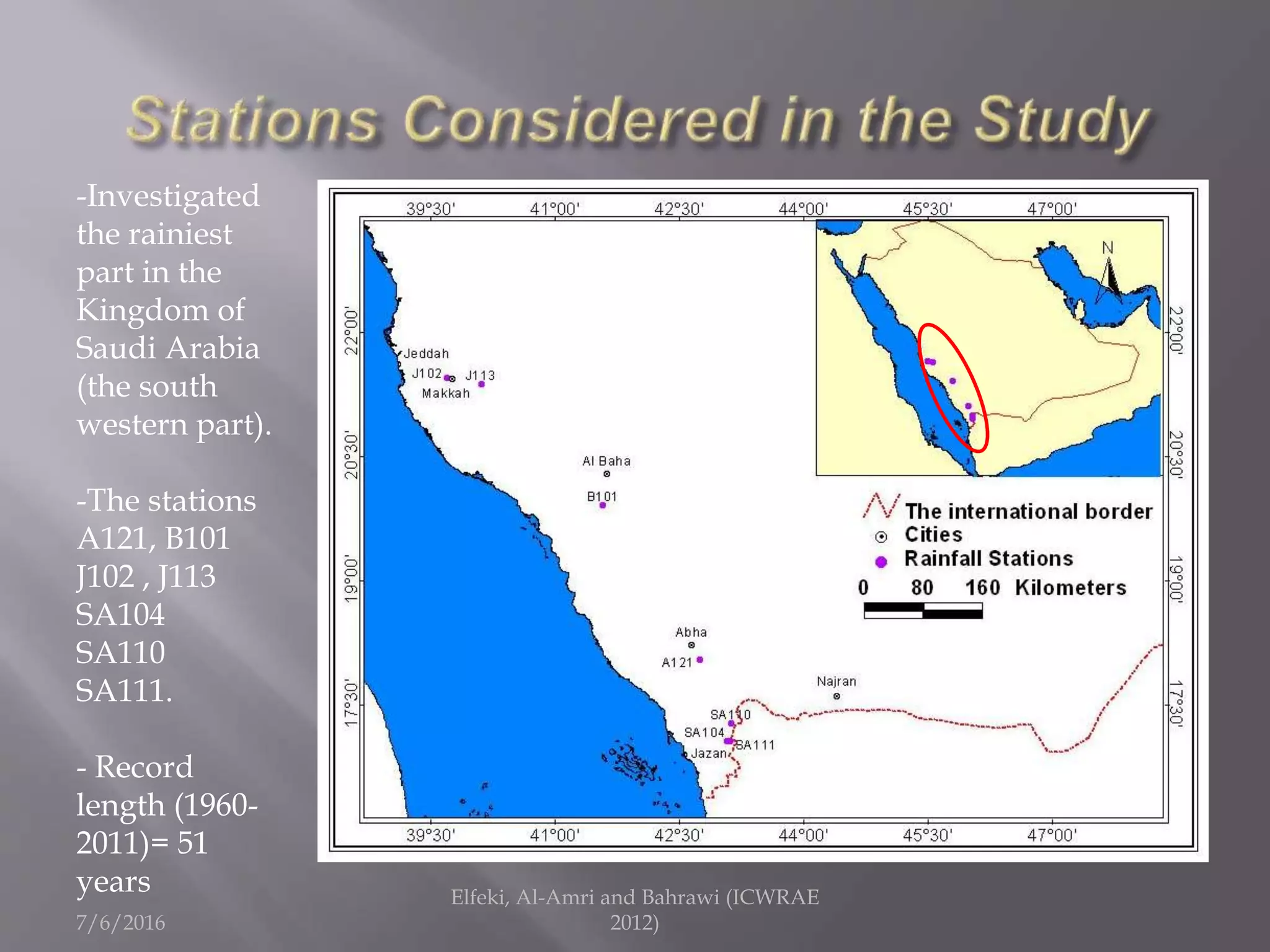
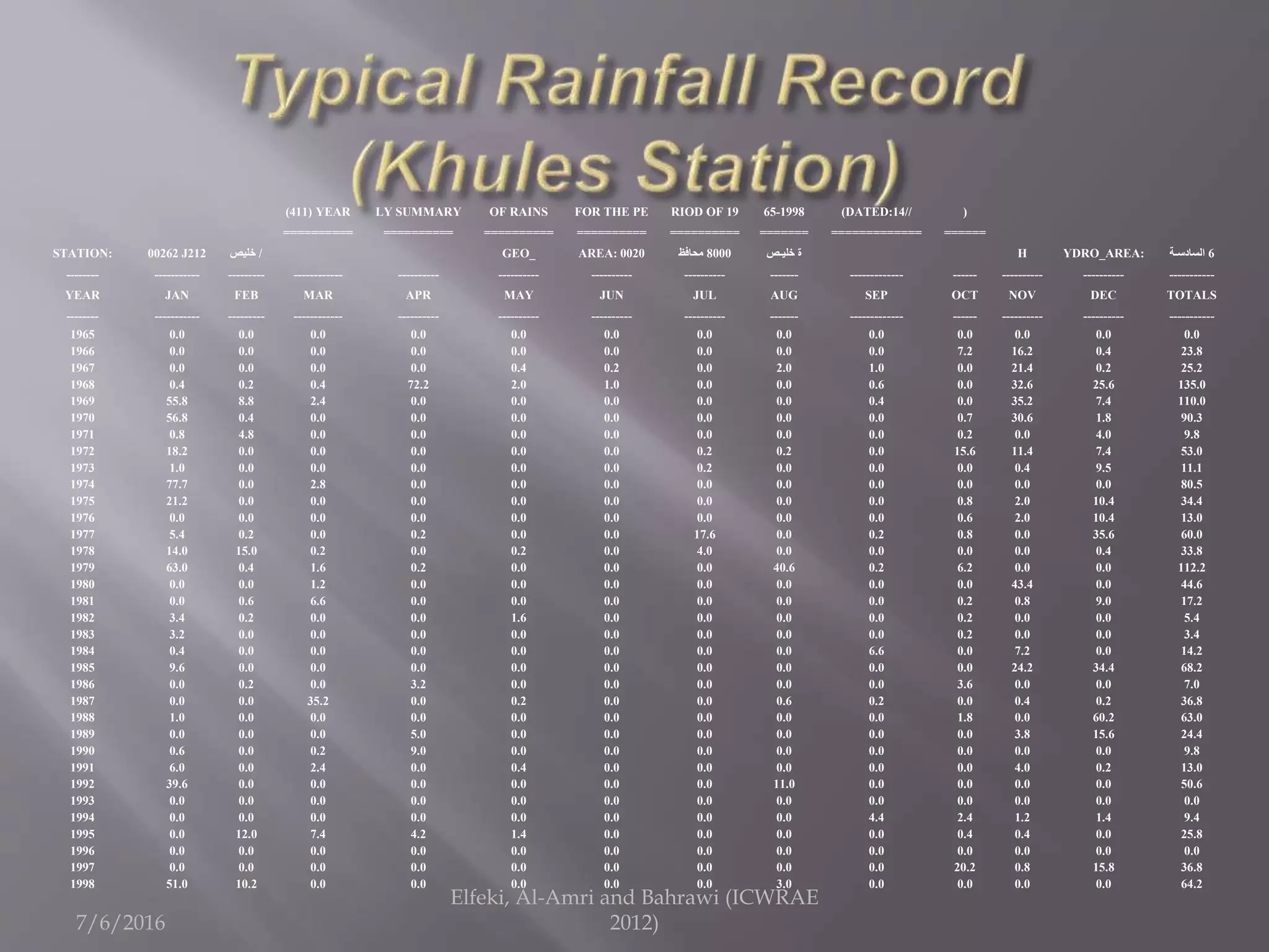
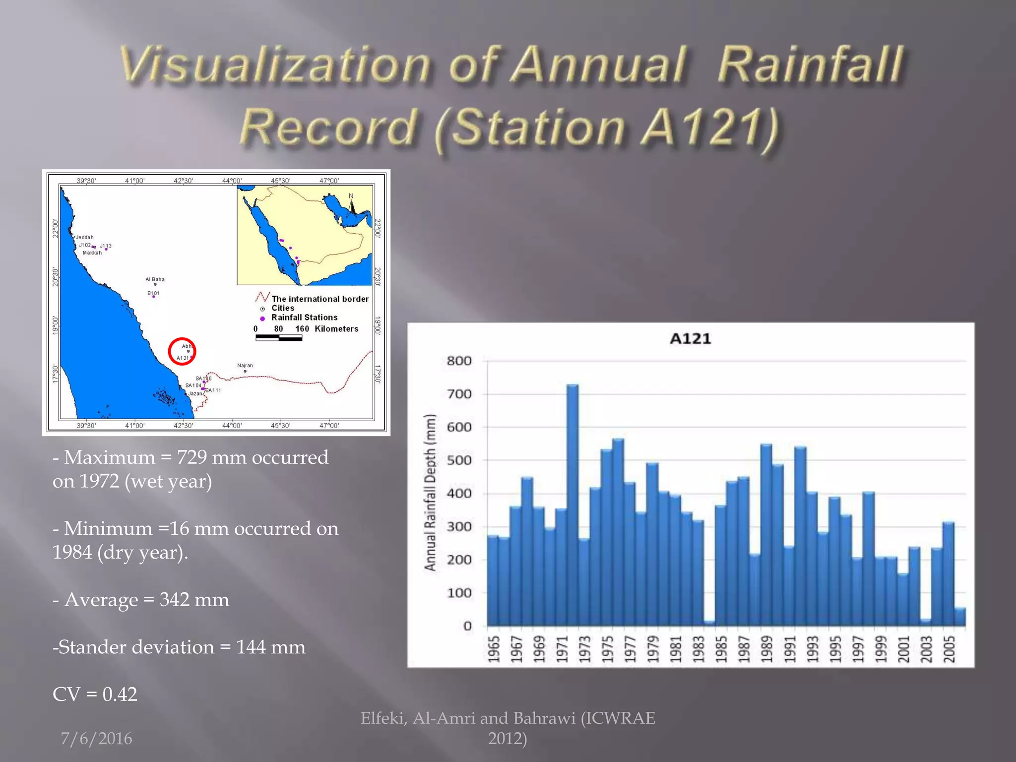
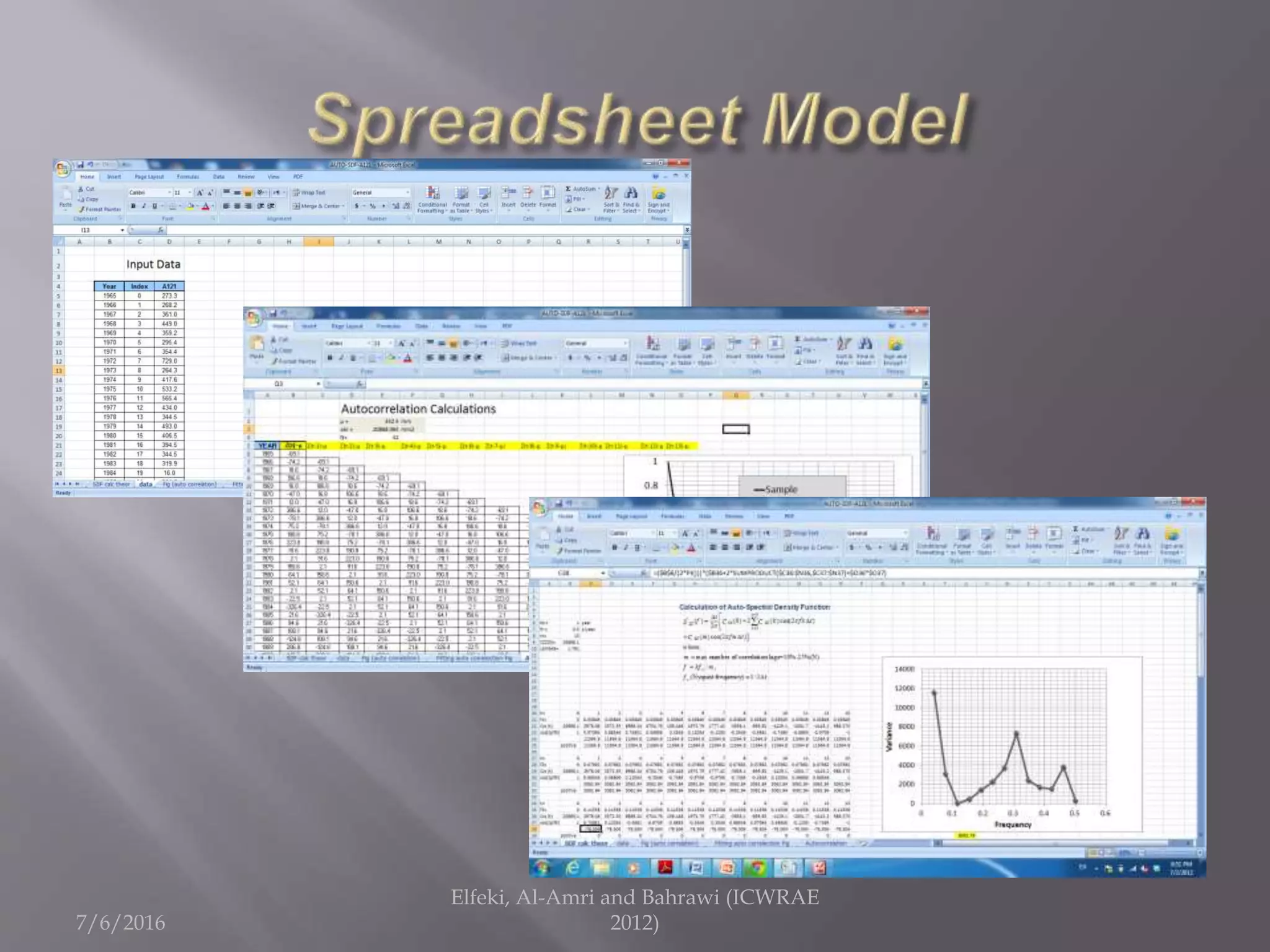
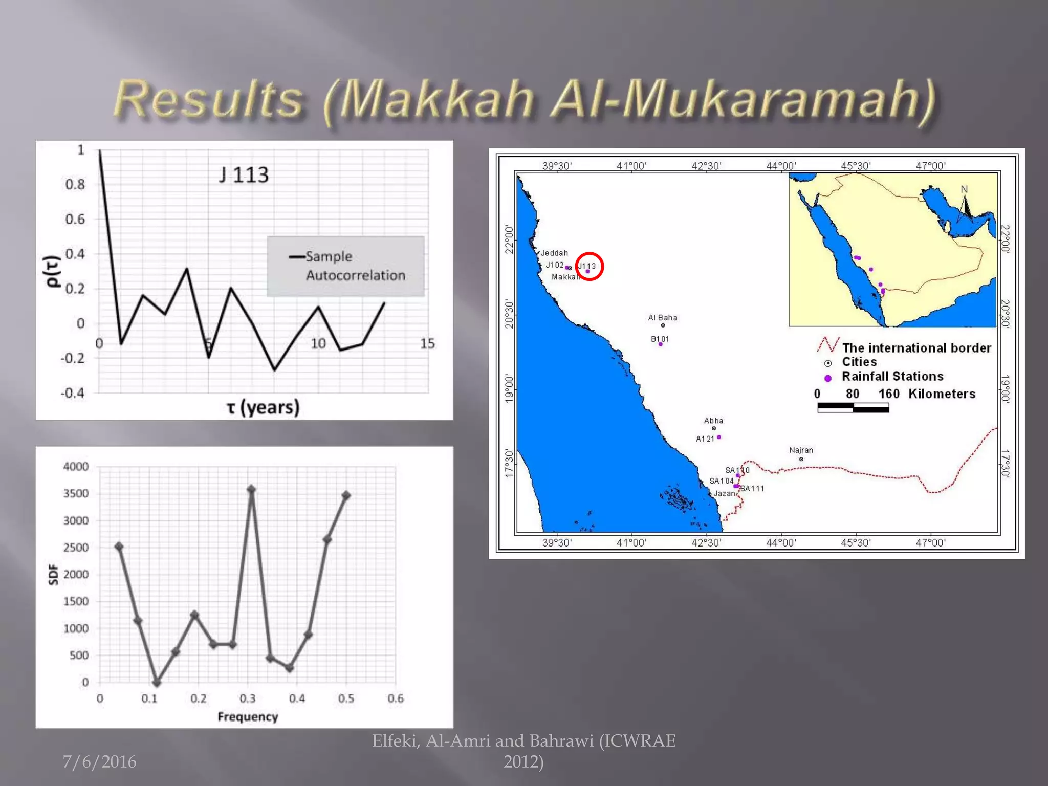
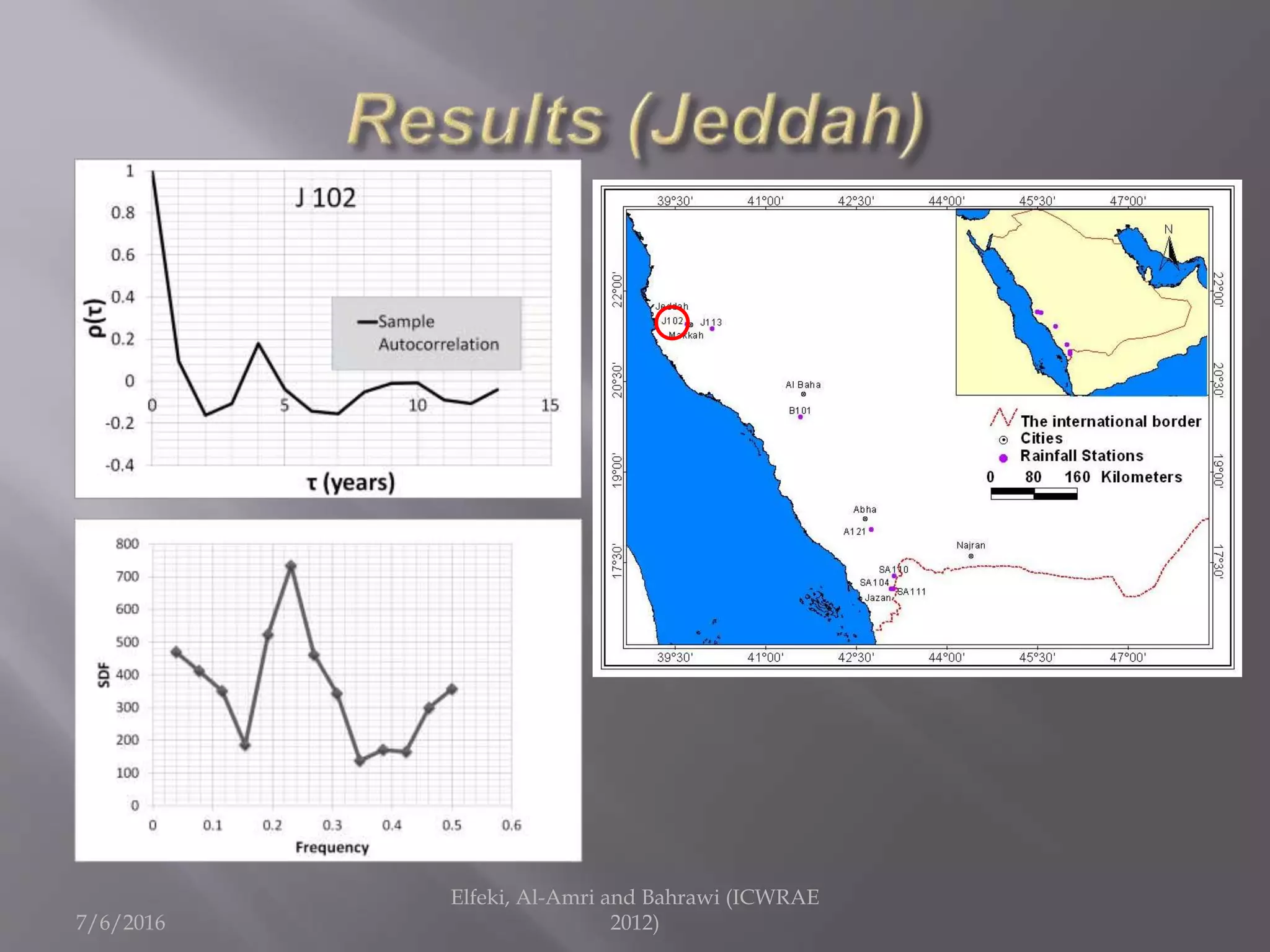
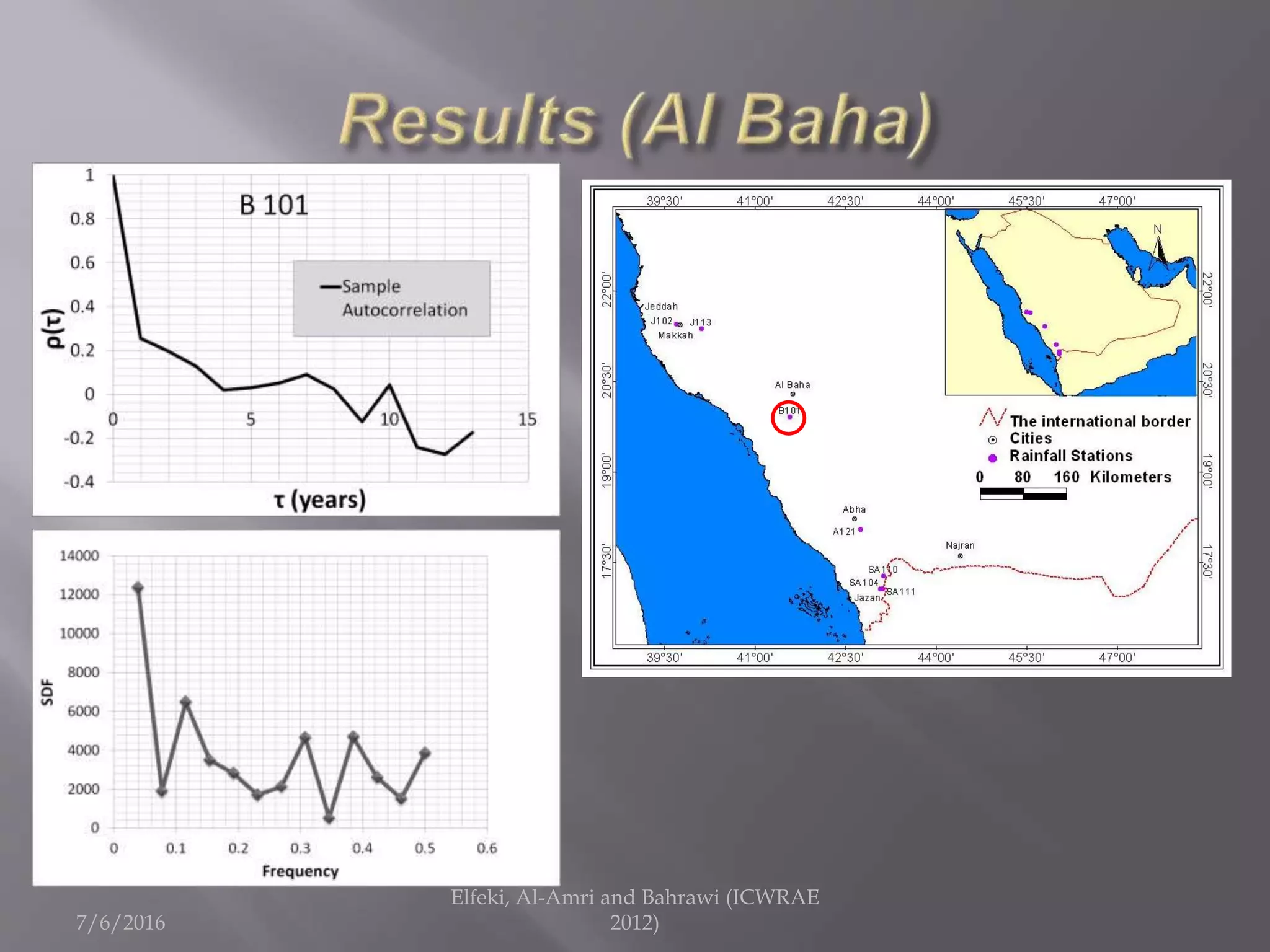
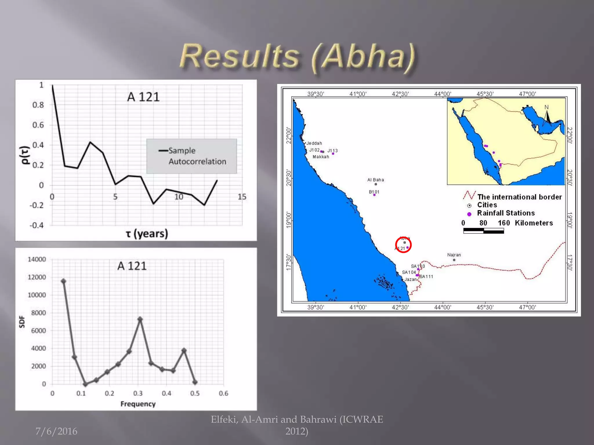
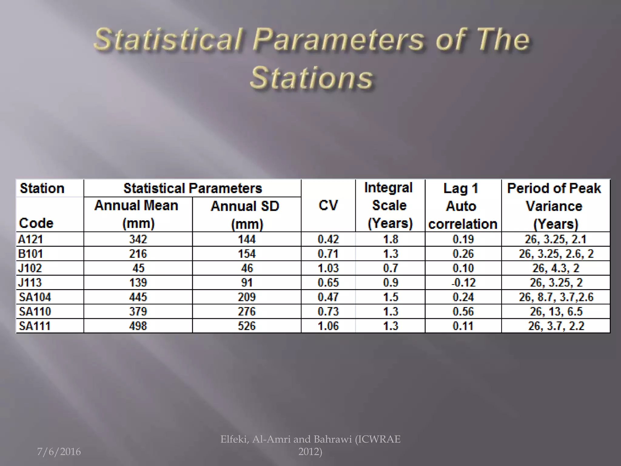
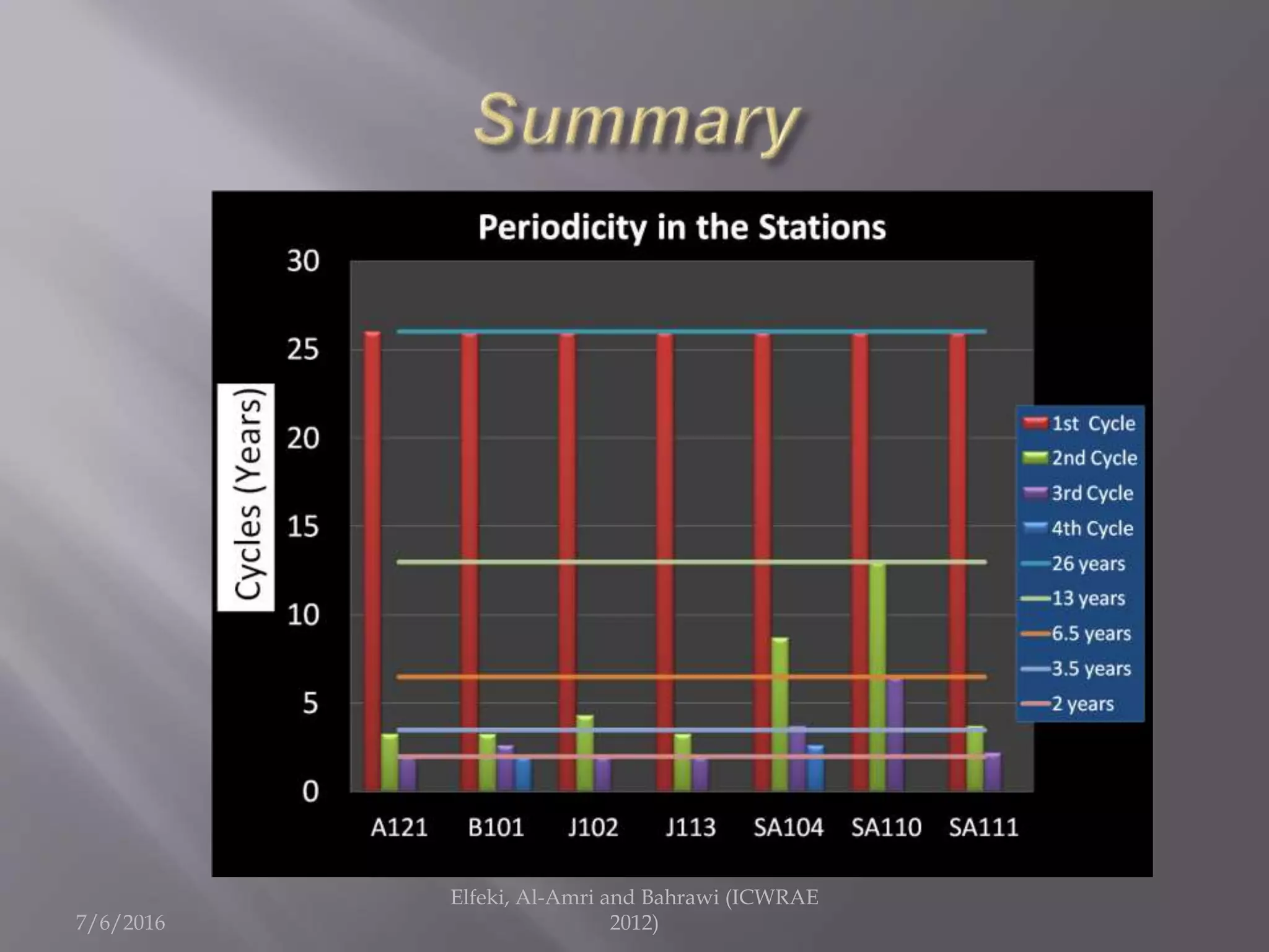
7/6/2016
Dept. of Hydrology and Water Resources Management
,Faculty of Meteorology, Environment & Arid Land
Agriculture, King Abdulaziz University , P.O. Box
80208 Jeddah 21589 Saudi Arabia
Elfeki, Al-Amri and Bahrawi (ICWRAE
2012)
Amro Elfeki, Nassir Al-Amri and Jarbou Bahrawi
 Research Objectives
 Typical Annual Rainfall Station Record
 Methodology and Model Development
 Results
 Conclusions
 Outlook
7/6/2016
Elfeki, Al-Amri and Bahrawi (ICWRAE
2012)
 Understanding the annual rainfall climate
variability in Saudi Arabia.
 Extraction of the modes of variations in the
annual rainfall record.
 Setting up an in-house tool (A spreadsheet
model) to perform analysis of the annual
rainfall variability and can be easily updated
once more data is available.
7/6/2016
Elfeki, Al-Amri and Bahrawi (ICWRAE
2012)
7/6/2016
Elfeki, Al-Amri and Bahrawi (ICWRAE
2012)
-Investigated
the rainiest
part in the
Kingdom of
Saudi Arabia
(the south
western part).
-The stations
A121, B101
J102 , J113
SA104
SA110
SA111.
- Record
length (1960-
2011)= 51
years
7/6/2016
Elfeki, Al-Amri and Bahrawi (ICWRAE
2012)
(411) YEAR LY SUMMARY OF RAINS FOR THE PE RIOD OF 19 65-1998 (DATED:14// )
========== ========== ========== ========== ========== ======= ============= ======
STATION: 00262 J212 /‫خليص‬ GEO_ AREA: 0020 8000‫محافظ‬ ‫خليـص‬ ‫ة‬ H YDRO_AREA: 6‫السادسـة‬
-------- ----------- --------- ------------ ---------- ---------- ---------- ---------- ------- ------------- ------ ---------- ---------- -----------
YEAR JAN FEB MAR APR MAY JUN JUL AUG SEP OCT NOV DEC TOTALS
-------- ----------- --------- ------------ ---------- ---------- ---------- ---------- ------- ------------- ------ ---------- ---------- -----------
1965 0.0 0.0 0.0 0.0 0.0 0.0 0.0 0.0 0.0 0.0 0.0 0.0 0.0
1966 0.0 0.0 0.0 0.0 0.0 0.0 0.0 0.0 0.0 7.2 16.2 0.4 23.8
1967 0.0 0.0 0.0 0.0 0.4 0.2 0.0 2.0 1.0 0.0 21.4 0.2 25.2
1968 0.4 0.2 0.4 72.2 2.0 1.0 0.0 0.0 0.6 0.0 32.6 25.6 135.0
1969 55.8 8.8 2.4 0.0 0.0 0.0 0.0 0.0 0.4 0.0 35.2 7.4 110.0
1970 56.8 0.4 0.0 0.0 0.0 0.0 0.0 0.0 0.0 0.7 30.6 1.8 90.3
1971 0.8 4.8 0.0 0.0 0.0 0.0 0.0 0.0 0.0 0.2 0.0 4.0 9.8
1972 18.2 0.0 0.0 0.0 0.0 0.0 0.2 0.2 0.0 15.6 11.4 7.4 53.0
1973 1.0 0.0 0.0 0.0 0.0 0.0 0.2 0.0 0.0 0.0 0.4 9.5 11.1
1974 77.7 0.0 2.8 0.0 0.0 0.0 0.0 0.0 0.0 0.0 0.0 0.0 80.5
1975 21.2 0.0 0.0 0.0 0.0 0.0 0.0 0.0 0.0 0.8 2.0 10.4 34.4
1976 0.0 0.0 0.0 0.0 0.0 0.0 0.0 0.0 0.0 0.6 2.0 10.4 13.0
1977 5.4 0.2 0.0 0.2 0.0 0.0 17.6 0.0 0.2 0.8 0.0 35.6 60.0
1978 14.0 15.0 0.2 0.0 0.2 0.0 4.0 0.0 0.0 0.0 0.0 0.4 33.8
1979 63.0 0.4 1.6 0.2 0.0 0.0 0.0 40.6 0.2 6.2 0.0 0.0 112.2
1980 0.0 0.0 1.2 0.0 0.0 0.0 0.0 0.0 0.0 0.0 43.4 0.0 44.6
1981 0.0 0.6 6.6 0.0 0.0 0.0 0.0 0.0 0.0 0.2 0.8 9.0 17.2
1982 3.4 0.2 0.0 0.0 1.6 0.0 0.0 0.0 0.0 0.2 0.0 0.0 5.4
1983 3.2 0.0 0.0 0.0 0.0 0.0 0.0 0.0 0.0 0.2 0.0 0.0 3.4
1984 0.4 0.0 0.0 0.0 0.0 0.0 0.0 0.0 6.6 0.0 7.2 0.0 14.2
1985 9.6 0.0 0.0 0.0 0.0 0.0 0.0 0.0 0.0 0.0 24.2 34.4 68.2
1986 0.0 0.2 0.0 3.2 0.0 0.0 0.0 0.0 0.0 3.6 0.0 0.0 7.0
1987 0.0 0.0 35.2 0.0 0.2 0.0 0.0 0.6 0.2 0.0 0.4 0.2 36.8
1988 1.0 0.0 0.0 0.0 0.0 0.0 0.0 0.0 0.0 1.8 0.0 60.2 63.0
1989 0.0 0.0 0.0 5.0 0.0 0.0 0.0 0.0 0.0 0.0 3.8 15.6 24.4
1990 0.6 0.0 0.2 9.0 0.0 0.0 0.0 0.0 0.0 0.0 0.0 0.0 9.8
1991 6.0 0.0 2.4 0.0 0.4 0.0 0.0 0.0 0.0 0.0 4.0 0.2 13.0
1992 39.6 0.0 0.0 0.0 0.0 0.0 0.0 11.0 0.0 0.0 0.0 0.0 50.6
1993 0.0 0.0 0.0 0.0 0.0 0.0 0.0 0.0 0.0 0.0 0.0 0.0 0.0
1994 0.0 0.0 0.0 0.0 0.0 0.0 0.0 0.0 4.4 2.4 1.2 1.4 9.4
1995 0.0 12.0 7.4 4.2 1.4 0.0 0.0 0.0 0.0 0.4 0.4 0.0 25.8
1996 0.0 0.0 0.0 0.0 0.0 0.0 0.0 0.0 0.0 0.0 0.0 0.0 0.0
1997 0.0 0.0 0.0 0.0 0.0 0.0 0.0 0.0 0.0 20.2 0.8 15.8 36.8
1998 51.0 10.2 0.0 0.0 0.0 0.0 0.0 3.0 0.0 0.0 0.0 0.0 64.2
7/6/2016
Elfeki, Al-Amri and Bahrawi (ICWRAE
2012)
- Maximum = 729 mm occurred
on 1972 (wet year)
- Minimum =16 mm occurred on
1984 (dry year).
- Average = 342 mm
-Stander deviation = 144 mm
CV = 0.42
 Methodology: Use of the autocorrelation and the
spectral density functions to examine the
modes of variation in the annual rainfall data.
 Model Development: Develop a spreadsheet
model to estimate both the autocorrelation and
the spectral density functions from the annual
data and extraction of the modes of variations.
7/6/2016
Elfeki, Al-Amri and Bahrawi (ICWRAE
2012)
7/6/2016
Elfeki, Al-Amri and Bahrawi (ICWRAE
2012)
 
2
( ), ( )
( )ZZ
z
Cov Z t Z t




ZZ
(0) 1
( ) 0
( ) = (- )
ZZ
ZZ
ZZ
=
=


  

Properties of stationary stochastic process maybe represented in a time domain which is
represented by the autocorrelation function of the lag τ. The autocorrelation function, , is
expressed as,
( )Z t ( )Z t 
2
z
 ( ), ( )Cov Z t Z t
is the variance of the stochastic process
are the stochastic process at two locations separated by a lag τ
is the covariance of the stochastic process at lag τ, which is given by,
( )
1
1
( ( ), ( )) ( ) - ( ) -
( )
n
j j
j
Cov Z t Z t Z Z Z Zt t
n

 
 
       + +
7/6/2016
Elfeki, Al-Amri and Bahrawi (ICWRAE
2012)
2*1 1
( ) lim ( ). ( ) lim | ( ) |zz
L L
f z f z f z fS
L L 
   
where, L is the length of the signal in the
frequency domain,
the over bar means a sample time average, and
z(f) is Fourier transform of the process Z(t),
which is expressed as,
- 21
( ) ( )
2
i ft
z f Z t dte




 
and z*(f) is the conjugate of z(f) and f is the angular frequency.
Properties of the Auto-power spectrum are formulated as,
2
-
( ) 0
( )
( ) ( )
zz
zz z
zz zz
fS
f d fS
f fS S





 

7/6/2016
Elfeki, Al-Amri and Bahrawi (ICWRAE
2012)
- 2
-
2
-
2
-
1
( ) ( )
2
( ) ( )
(0) ( )
i f
zz zz
i f
zz zz
zz zz Z
f dS C e
f d fC S e
f d fC S
 
 
 











 



The covariance functions and spectral density functions are Fourier
transform pairs. This can be expressed in mathematical forms using
Wiener-Khinchin relationships
7/6/2016
Elfeki, Al-Amri and Bahrawi (ICWRAE
2012)
0
1
( ) ( )cos(2 )zz zzf C f dS    


 
1
1
ˆ ( ) (0) 2 ( )cos(2 ) ( )cos(2 )
2
m
zz zz zzzz
k
t
f C C k fk t C m fm tS  



  
     
 

,
max number of correlation lags=10%-25%(N)
/ ,
(Nyquist frequency) 1/ 2
0,1,2...,
n
n
where
m
f kf m
f t
k m


 

7/6/2016
Elfeki, Al-Amri and Bahrawi (ICWRAE
2012)
7/6/2016
Elfeki, Al-Amri and Bahrawi (ICWRAE
2012)
7/6/2016
Elfeki, Al-Amri and Bahrawi (ICWRAE
2012)
7/6/2016
Elfeki, Al-Amri and Bahrawi (ICWRAE
2012)
7/6/2016
Elfeki, Al-Amri and Bahrawi (ICWRAE
2012)
7/6/2016
Elfeki, Al-Amri and Bahrawi (ICWRAE
2012)
7/6/2016
Elfeki, Al-Amri and Bahrawi (ICWRAE
2012)
7/6/2016
Elfeki, Al-Amri and Bahrawi (ICWRAE
2012)
7/6/2016
Elfeki, Al-Amri and Bahrawi (ICWRAE
2012)
7/6/2016
Elfeki, Al-Amri and Bahrawi (ICWRAE
2012)
 Multiple temporal scales were obtained with
relatively significant variance and it is therefore
difficult to identify the organized structures in
the spectra except the 26 and 2 years cycles are
common for all stations.
 The significant cycles from all stations are 26,
13, 6.5, 3.5 and 2 years.
 Continuous recoding is a must to enable
reliable analysis.
7/6/2016
Elfeki, Al-Amri and Bahrawi (ICWRAE
2012)
 One of the applications of this study is to build
time series models from the available data. The
models are based on reconstruction of the
significant ‘signals’ from the data.
 Further analysis is needed to other stations in
the Kingdom.
7/6/2016
Elfeki, Al-Amri and Bahrawi (ICWRAE
2012)

Analysis of Annual Rainfall Climate Variability in Saudi Arabia by Using Spectral Density Function.

  • 1.
    7/6/2016 Dept. of Hydrologyand Water Resources Management ,Faculty of Meteorology, Environment & Arid Land Agriculture, King Abdulaziz University , P.O. Box 80208 Jeddah 21589 Saudi Arabia Elfeki, Al-Amri and Bahrawi (ICWRAE 2012) Amro Elfeki, Nassir Al-Amri and Jarbou Bahrawi
  • 2.
     Research Objectives Typical Annual Rainfall Station Record  Methodology and Model Development  Results  Conclusions  Outlook 7/6/2016 Elfeki, Al-Amri and Bahrawi (ICWRAE 2012)
  • 3.
     Understanding theannual rainfall climate variability in Saudi Arabia.  Extraction of the modes of variations in the annual rainfall record.  Setting up an in-house tool (A spreadsheet model) to perform analysis of the annual rainfall variability and can be easily updated once more data is available. 7/6/2016 Elfeki, Al-Amri and Bahrawi (ICWRAE 2012)
  • 4.
    7/6/2016 Elfeki, Al-Amri andBahrawi (ICWRAE 2012) -Investigated the rainiest part in the Kingdom of Saudi Arabia (the south western part). -The stations A121, B101 J102 , J113 SA104 SA110 SA111. - Record length (1960- 2011)= 51 years
  • 5.
    7/6/2016 Elfeki, Al-Amri andBahrawi (ICWRAE 2012) (411) YEAR LY SUMMARY OF RAINS FOR THE PE RIOD OF 19 65-1998 (DATED:14// ) ========== ========== ========== ========== ========== ======= ============= ====== STATION: 00262 J212 /‫خليص‬ GEO_ AREA: 0020 8000‫محافظ‬ ‫خليـص‬ ‫ة‬ H YDRO_AREA: 6‫السادسـة‬ -------- ----------- --------- ------------ ---------- ---------- ---------- ---------- ------- ------------- ------ ---------- ---------- ----------- YEAR JAN FEB MAR APR MAY JUN JUL AUG SEP OCT NOV DEC TOTALS -------- ----------- --------- ------------ ---------- ---------- ---------- ---------- ------- ------------- ------ ---------- ---------- ----------- 1965 0.0 0.0 0.0 0.0 0.0 0.0 0.0 0.0 0.0 0.0 0.0 0.0 0.0 1966 0.0 0.0 0.0 0.0 0.0 0.0 0.0 0.0 0.0 7.2 16.2 0.4 23.8 1967 0.0 0.0 0.0 0.0 0.4 0.2 0.0 2.0 1.0 0.0 21.4 0.2 25.2 1968 0.4 0.2 0.4 72.2 2.0 1.0 0.0 0.0 0.6 0.0 32.6 25.6 135.0 1969 55.8 8.8 2.4 0.0 0.0 0.0 0.0 0.0 0.4 0.0 35.2 7.4 110.0 1970 56.8 0.4 0.0 0.0 0.0 0.0 0.0 0.0 0.0 0.7 30.6 1.8 90.3 1971 0.8 4.8 0.0 0.0 0.0 0.0 0.0 0.0 0.0 0.2 0.0 4.0 9.8 1972 18.2 0.0 0.0 0.0 0.0 0.0 0.2 0.2 0.0 15.6 11.4 7.4 53.0 1973 1.0 0.0 0.0 0.0 0.0 0.0 0.2 0.0 0.0 0.0 0.4 9.5 11.1 1974 77.7 0.0 2.8 0.0 0.0 0.0 0.0 0.0 0.0 0.0 0.0 0.0 80.5 1975 21.2 0.0 0.0 0.0 0.0 0.0 0.0 0.0 0.0 0.8 2.0 10.4 34.4 1976 0.0 0.0 0.0 0.0 0.0 0.0 0.0 0.0 0.0 0.6 2.0 10.4 13.0 1977 5.4 0.2 0.0 0.2 0.0 0.0 17.6 0.0 0.2 0.8 0.0 35.6 60.0 1978 14.0 15.0 0.2 0.0 0.2 0.0 4.0 0.0 0.0 0.0 0.0 0.4 33.8 1979 63.0 0.4 1.6 0.2 0.0 0.0 0.0 40.6 0.2 6.2 0.0 0.0 112.2 1980 0.0 0.0 1.2 0.0 0.0 0.0 0.0 0.0 0.0 0.0 43.4 0.0 44.6 1981 0.0 0.6 6.6 0.0 0.0 0.0 0.0 0.0 0.0 0.2 0.8 9.0 17.2 1982 3.4 0.2 0.0 0.0 1.6 0.0 0.0 0.0 0.0 0.2 0.0 0.0 5.4 1983 3.2 0.0 0.0 0.0 0.0 0.0 0.0 0.0 0.0 0.2 0.0 0.0 3.4 1984 0.4 0.0 0.0 0.0 0.0 0.0 0.0 0.0 6.6 0.0 7.2 0.0 14.2 1985 9.6 0.0 0.0 0.0 0.0 0.0 0.0 0.0 0.0 0.0 24.2 34.4 68.2 1986 0.0 0.2 0.0 3.2 0.0 0.0 0.0 0.0 0.0 3.6 0.0 0.0 7.0 1987 0.0 0.0 35.2 0.0 0.2 0.0 0.0 0.6 0.2 0.0 0.4 0.2 36.8 1988 1.0 0.0 0.0 0.0 0.0 0.0 0.0 0.0 0.0 1.8 0.0 60.2 63.0 1989 0.0 0.0 0.0 5.0 0.0 0.0 0.0 0.0 0.0 0.0 3.8 15.6 24.4 1990 0.6 0.0 0.2 9.0 0.0 0.0 0.0 0.0 0.0 0.0 0.0 0.0 9.8 1991 6.0 0.0 2.4 0.0 0.4 0.0 0.0 0.0 0.0 0.0 4.0 0.2 13.0 1992 39.6 0.0 0.0 0.0 0.0 0.0 0.0 11.0 0.0 0.0 0.0 0.0 50.6 1993 0.0 0.0 0.0 0.0 0.0 0.0 0.0 0.0 0.0 0.0 0.0 0.0 0.0 1994 0.0 0.0 0.0 0.0 0.0 0.0 0.0 0.0 4.4 2.4 1.2 1.4 9.4 1995 0.0 12.0 7.4 4.2 1.4 0.0 0.0 0.0 0.0 0.4 0.4 0.0 25.8 1996 0.0 0.0 0.0 0.0 0.0 0.0 0.0 0.0 0.0 0.0 0.0 0.0 0.0 1997 0.0 0.0 0.0 0.0 0.0 0.0 0.0 0.0 0.0 20.2 0.8 15.8 36.8 1998 51.0 10.2 0.0 0.0 0.0 0.0 0.0 3.0 0.0 0.0 0.0 0.0 64.2
  • 6.
    7/6/2016 Elfeki, Al-Amri andBahrawi (ICWRAE 2012) - Maximum = 729 mm occurred on 1972 (wet year) - Minimum =16 mm occurred on 1984 (dry year). - Average = 342 mm -Stander deviation = 144 mm CV = 0.42
  • 7.
     Methodology: Useof the autocorrelation and the spectral density functions to examine the modes of variation in the annual rainfall data.  Model Development: Develop a spreadsheet model to estimate both the autocorrelation and the spectral density functions from the annual data and extraction of the modes of variations. 7/6/2016 Elfeki, Al-Amri and Bahrawi (ICWRAE 2012)
  • 8.
    7/6/2016 Elfeki, Al-Amri andBahrawi (ICWRAE 2012)   2 ( ), ( ) ( )ZZ z Cov Z t Z t     ZZ (0) 1 ( ) 0 ( ) = (- ) ZZ ZZ ZZ = =       Properties of stationary stochastic process maybe represented in a time domain which is represented by the autocorrelation function of the lag τ. The autocorrelation function, , is expressed as, ( )Z t ( )Z t  2 z  ( ), ( )Cov Z t Z t is the variance of the stochastic process are the stochastic process at two locations separated by a lag τ is the covariance of the stochastic process at lag τ, which is given by, ( ) 1 1 ( ( ), ( )) ( ) - ( ) - ( ) n j j j Cov Z t Z t Z Z Z Zt t n             + +
  • 9.
    7/6/2016 Elfeki, Al-Amri andBahrawi (ICWRAE 2012) 2*1 1 ( ) lim ( ). ( ) lim | ( ) |zz L L f z f z f z fS L L      where, L is the length of the signal in the frequency domain, the over bar means a sample time average, and z(f) is Fourier transform of the process Z(t), which is expressed as, - 21 ( ) ( ) 2 i ft z f Z t dte       and z*(f) is the conjugate of z(f) and f is the angular frequency. Properties of the Auto-power spectrum are formulated as, 2 - ( ) 0 ( ) ( ) ( ) zz zz z zz zz fS f d fS f fS S        
  • 10.
    7/6/2016 Elfeki, Al-Amri andBahrawi (ICWRAE 2012) - 2 - 2 - 2 - 1 ( ) ( ) 2 ( ) ( ) (0) ( ) i f zz zz i f zz zz zz zz Z f dS C e f d fC S e f d fC S                       The covariance functions and spectral density functions are Fourier transform pairs. This can be expressed in mathematical forms using Wiener-Khinchin relationships
  • 11.
    7/6/2016 Elfeki, Al-Amri andBahrawi (ICWRAE 2012) 0 1 ( ) ( )cos(2 )zz zzf C f dS         1 1 ˆ ( ) (0) 2 ( )cos(2 ) ( )cos(2 ) 2 m zz zz zzzz k t f C C k fk t C m fm tS                  , max number of correlation lags=10%-25%(N) / , (Nyquist frequency) 1/ 2 0,1,2..., n n where m f kf m f t k m     
  • 12.
    7/6/2016 Elfeki, Al-Amri andBahrawi (ICWRAE 2012)
  • 13.
    7/6/2016 Elfeki, Al-Amri andBahrawi (ICWRAE 2012)
  • 14.
    7/6/2016 Elfeki, Al-Amri andBahrawi (ICWRAE 2012)
  • 15.
    7/6/2016 Elfeki, Al-Amri andBahrawi (ICWRAE 2012)
  • 16.
    7/6/2016 Elfeki, Al-Amri andBahrawi (ICWRAE 2012)
  • 17.
    7/6/2016 Elfeki, Al-Amri andBahrawi (ICWRAE 2012)
  • 18.
    7/6/2016 Elfeki, Al-Amri andBahrawi (ICWRAE 2012)
  • 19.
    7/6/2016 Elfeki, Al-Amri andBahrawi (ICWRAE 2012)
  • 20.
    7/6/2016 Elfeki, Al-Amri andBahrawi (ICWRAE 2012)
  • 21.
    7/6/2016 Elfeki, Al-Amri andBahrawi (ICWRAE 2012)
  • 22.
     Multiple temporalscales were obtained with relatively significant variance and it is therefore difficult to identify the organized structures in the spectra except the 26 and 2 years cycles are common for all stations.  The significant cycles from all stations are 26, 13, 6.5, 3.5 and 2 years.  Continuous recoding is a must to enable reliable analysis. 7/6/2016 Elfeki, Al-Amri and Bahrawi (ICWRAE 2012)
  • 23.
     One ofthe applications of this study is to build time series models from the available data. The models are based on reconstruction of the significant ‘signals’ from the data.  Further analysis is needed to other stations in the Kingdom. 7/6/2016 Elfeki, Al-Amri and Bahrawi (ICWRAE 2012)