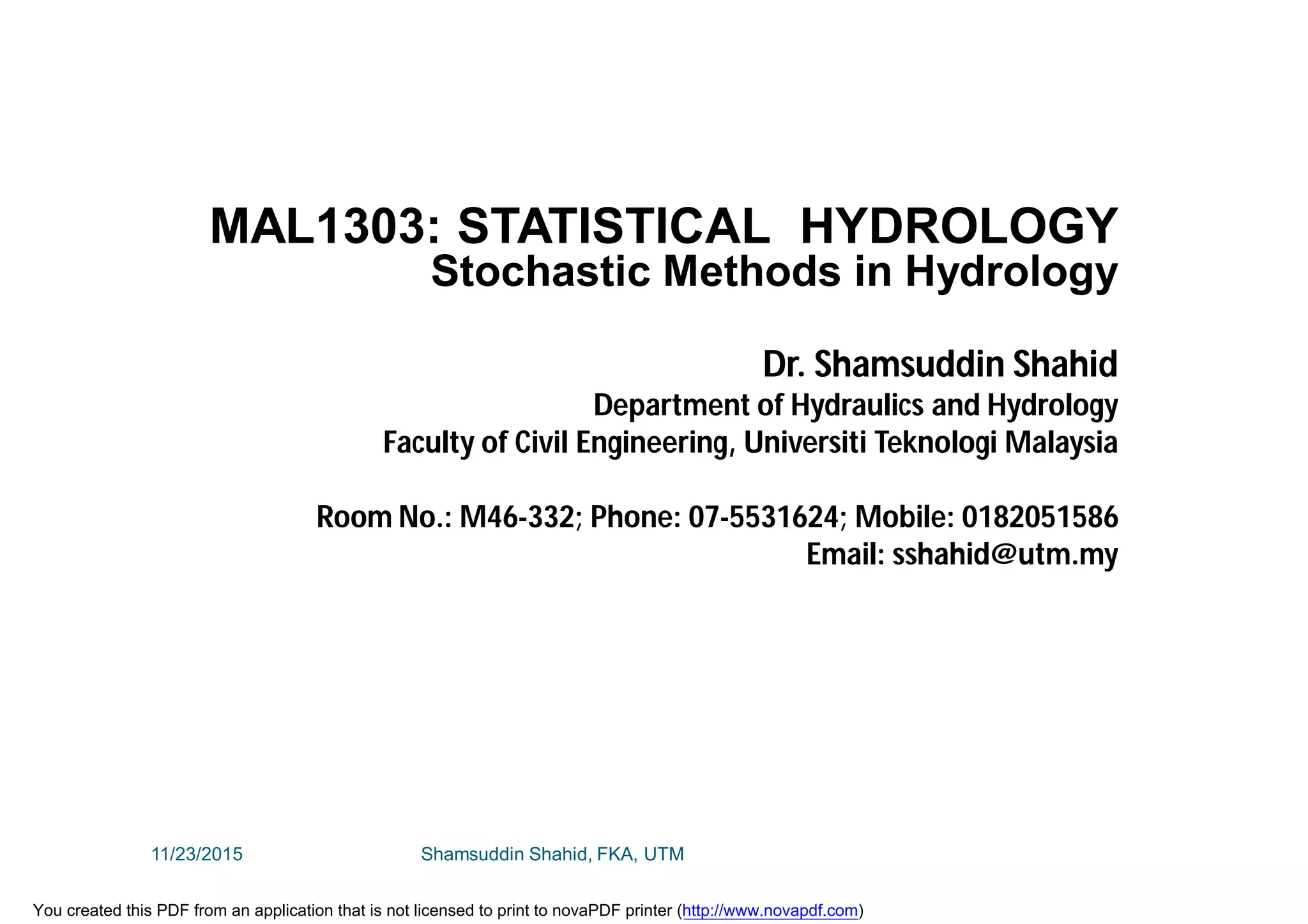
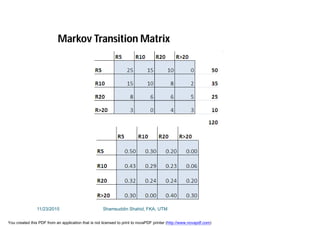
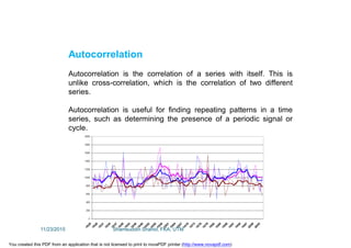
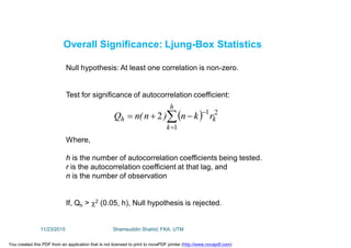
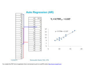
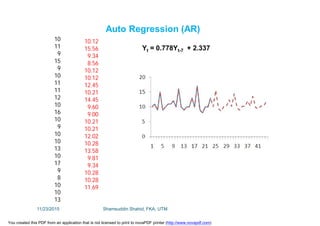
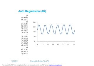
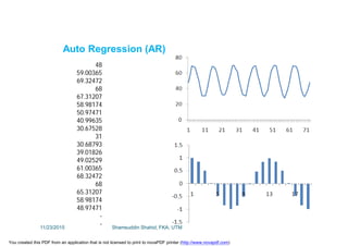
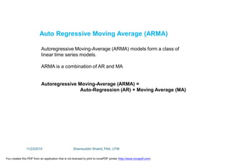
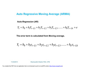
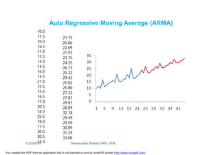
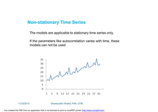
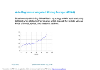
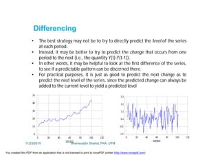
This document discusses stochastic methods in hydrology, specifically Markov transition matrices and cumulative distribution functions. It describes how to calculate daily monsoon rainfall using a Markov chain model with four rainfall classes. The initial condition and transition probabilities are given. It also discusses stationary time series, linear stochastic models including moving averages, autoregressive models and autoregressive moving average models. Double moving averages are presented to remove trends and improve forecasts.

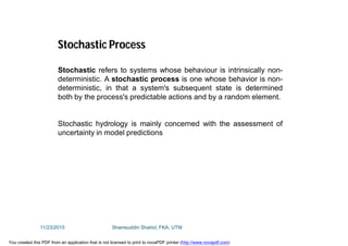
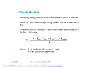
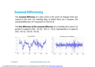
![For four class, there will be four cumulative distribution functions.
Cumulative distribution functions for each class is calculated as,
Fj (x) = P [next day rainfall < x; when rainfall today belongs to class Cj].
For Example,
FR5(x) = P [next day rainfall < x; when rainfall today belongs to class R5].
Cumulative Distribution Functions
11/23/2015 Shamsuddin Shahid, FKA, UTM
You created this PDF from an application that is not licensed to print to novaPDF printer (http://www.novapdf.com)](https://image.slidesharecdn.com/shahid-lecture-12-mkag1273-151123082934-lva1-app6892/85/Shahid-Lecture-12-MKAG1273-3-320.jpg)
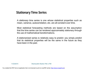
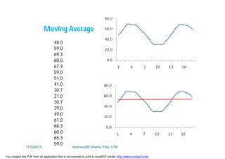
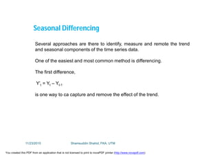
![Fj (x) = P [next day rainfall < x;
when rainfall today belongs to class Cj].
For Example:
FR5(x) = P [next day rainfall < x;
when rainfall today belongs to class R5].
P [next day rainfall < 5] = 2
P [next day rainfall < 4] = 2
P [next day rainfall < 3] = 2
P [next day rainfall < 2] = 1
P [next day rainfall < 1] = 1
Rainfall
10
5
1
6
23
4
3
2
0
20
5
2
3
0
4
3
1
0
Cumulative Distribution Functions
11/23/2015 Shamsuddin Shahid, FKA, UTM
You created this PDF from an application that is not licensed to print to novaPDF printer (http://www.novapdf.com)](https://image.slidesharecdn.com/shahid-lecture-12-mkag1273-151123082934-lva1-app6892/85/Shahid-Lecture-12-MKAG1273-4-320.jpg)
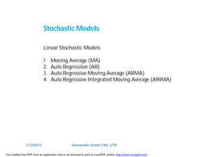
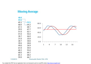
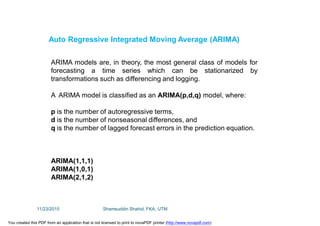
![FR5(x) = P [next day rainfall < x;
when rainfall today belongs to class R5].
P [next day rainfall < 5] = 2
P [next day rainfall < 4] = 2
P [next day rainfall < 3] = 2
P [next day rainfall < 2] = 1
P [next day rainfall < 1] = 1
Cumulative Distribution Functions
Find the distribution
and distribution
parameters.
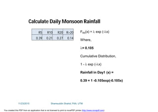
Consider, we found
distribution is
exponential,
FR5(x) = exp (-)
Where,
= 0.105
11/23/2015 Shamsuddin Shahid, FKA, UTM
You created this PDF from an application that is not licensed to print to novaPDF printer (http://www.novapdf.com)](https://image.slidesharecdn.com/shahid-lecture-12-mkag1273-151123082934-lva1-app6892/85/Shahid-Lecture-12-MKAG1273-5-320.jpg)
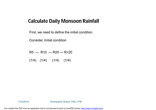
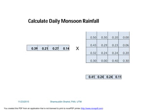
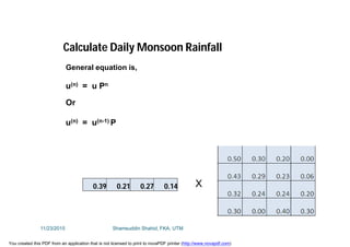
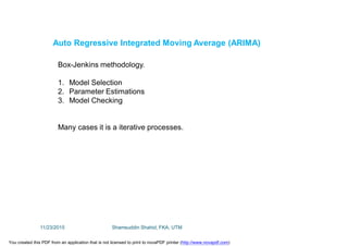
![Calculate Daily Monsoon Rainfall
(1/4) (1/4) (1/4) (1/4)
[0.25 0.25 0.25 0.25] X
0.39 0.21 0.27 0.14
11/23/2015 Shamsuddin Shahid, FKA, UTM
You created this PDF from an application that is not licensed to print to novaPDF printer (http://www.novapdf.com)](https://image.slidesharecdn.com/shahid-lecture-12-mkag1273-151123082934-lva1-app6892/85/Shahid-Lecture-12-MKAG1273-7-320.jpg)

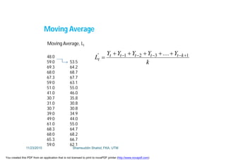
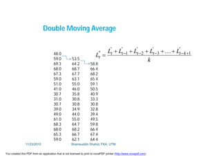
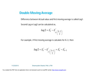
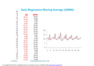
![Double Moving Average: Forecasting
Double moving average can be used for forecasting using following
formulas:
mbaF ttt 1
Where,
//
t
/
tt
//
t
/
t
/
tt
LL
k
b
and
]LL[La
1
2
11/23/2015 Shamsuddin Shahid, FKA, UTM
You created this PDF from an application that is not licensed to print to novaPDF printer (http://www.novapdf.com)](https://image.slidesharecdn.com/shahid-lecture-12-mkag1273-151123082934-lva1-app6892/85/Shahid-Lecture-12-MKAG1273-23-320.jpg)
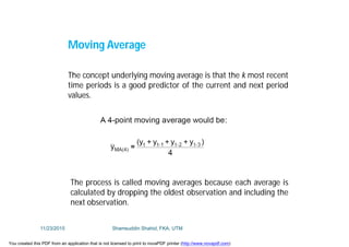
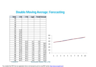
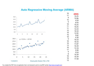
![Data L'(t) L"(t) Lag2 Trend Forecast Error
10.0
12.0 11.0
14.0 13.0 12.0 1.0 2.0
16.0 15.0 14.0 1.0 2.0 16.0 0.0
18.0 17.0 16.0 1.0 2.0 18.0 0.0
20.0 19.0 18.0 1.0 2.0 20.0 0.0
22.0 21.0 20.0 1.0 2.0 22.0 0.0
24.0 23.0 22.0 1.0 2.0 24.0 0.0
26.0 25.0 24.0 1.0 2.0 26.0 0.0
28.0 27.0 26.0 1.0 2.0 28.0 0.0
30.0 29.0 28.0 1.0 2.0 30.0 0.0
32.0 31.0 30.0 1.0 2.0 32.0 0.0
34.0 33.0 32.0 1.0 2.0 34.0 0.0
36.0 35.0 34.0 1.0 2.0 36.0 0.0
38.0 37.0 36.0 1.0 2.0 38.0 0.0
40.0 39.0 38.0 1.0 2.0 40.0 0.0
42.0 41.0 40.0 1.0 2.0 42.0 0.0
44.0 43.0 42.0 1.0 2.0 44.0 0.0
Double Moving Average: Forecasting
//
t
/
tt
//
t
/
t
/
tt
LL
k
b
and
]LL[La
1
2
ttt baF 1
11/23/2015 Shamsuddin Shahid, FKA, UTM
You created this PDF from an application that is not licensed to print to novaPDF printer (http://www.novapdf.com)](https://image.slidesharecdn.com/shahid-lecture-12-mkag1273-151123082934-lva1-app6892/85/Shahid-Lecture-12-MKAG1273-24-320.jpg)


![GoogleCTF 2016 [No Big Deal] Write-Up (ver.korean)](https://cdn.slidesharecdn.com/ss_thumbnails/googlectf2016nobigdealwrite-upver-160504191100-thumbnail.jpg?width=640&height=640&fit=bounds)


![time series.ppt [Autosaved].pdf](https://cdn.slidesharecdn.com/ss_thumbnails/timeseries-231013231623-6993e801-thumbnail.jpg?width=640&height=640&fit=bounds)