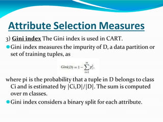
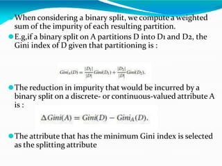
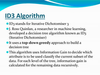
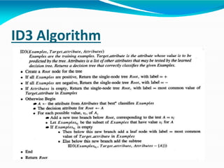
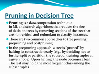
Subject Coordinator : Aakanksha Agrawal
Unit-3
Attribute Selection Measures
⚫An attribute selection measure is a heuristic for
selecting the splitting criterion that “best” separates a
given data partition, D, of class-labeled training tuples
into individual classes.
⚫Attribute selection measures are also known as
splitting rules because they determine how the
tuples at a given node are to be split.
⚫The attribute selection measure provides a ranking for
each attribute describing the given training tuples.
The attribute having the best score for the measure is
chosen as the splitting attribute for the given tuples
Attribute Selection Measures
⚫Three popular attribute selection measures
1) Information gain This attribute minimizes the
information needed to classify the tuples in the resulting
partitions and reflects the least randomness or “impurity”
in these partitions.
Such an approach minimizes the expected number of tests
needed to classify a given tuple and guarantees that a
simple (but not necessarily the simplest) tree is found
Let node N represent or hold the tuples of partition D. The
attribute with highest information gain is chosen as the
splitting attribute for node N.
⚫The expected information needed to classify a tuple in D is
given by :
where pi is the nonzero probability that an arbitrary tuple in
D belongs to class Ci and is estimated by |Ci,D|/|D|.
⚫A log function to the base 2 is used, because the
information is encoded in bits.
⚫Info(D) is just the average amount of information needed
to identify the class label of a tuple in D.
⚫Info(D) is also known as the entropy of D.
⚫ Suppose we were to partition the tuples in D on some attribute A
having v distinct values, {a1, a2,..., av }, as observed from the training
data
⚫ Attribute A can be used to split D into v partitions or subsets, {D1,
D2,..., Dv },
⚫ These partitions would correspond to the branches grown from node
N.
⚫ The expected information required to classify a tuple from D based
on the partitioning by A is given by :
The term |Dj | /|D| acts as the weight of the jth partition.
⚫ Information gain is defined as the difference between the original
information requirement (i.e., based on just the proportion of classes) and
the new requirement (i.e., obtained after partitioning on A).
⚫ The expected information needed to classify a tuple in D:
⚫Expected information needed to classify a tuple in D if the
tuples are partitioned according to age is :
⚫Hence, the gain in information from such a partitioning
would be Gain(age) = Info(D) − Infoage(D) = 0.940 −
0.694 = 0.246 bits.
⚫Gain(income) = 0.029 bits, Gain(student) = 0.151 bits,
and Gain(credit rating) = 0.048 bits. Because age has
the highest information gain among the attributes, it
is selected as the splitting attribute.
Attribute Selection Measures
2) Gain ratio The information gain measure is biased toward
tests with many outcomes. That is, it prefers to select
attributes having a large number of values
⚫ C4.5, a successor of ID3, uses an extension to information
gain known as gain ratio, which attempts to overcome this
bias.
⚫ It applies a kind of normalization to information gain
using a “split information” value defined analogously with
Info(D) as :
⚫This value represents the potential information generated
by splitting the training data set, D, into v partitions,
corresponding to the v outcomes of a test on attribute A.
⚫The gain ratio is defined as
⚫The attribute with the maximum gain ratio is selected as the
splitting attribute
⚫Tocompute the gain ratio of income,
⚫Gain(income) = 0.029.
⚫Therefore, GainRatio(income) = 0.029/1.557 = 0.019.
Attribute Selection Measures
3) Gini index The Gini index is used in CART.
⚫Gini index measures the impurity of D, a data partition or
set of training tuples, as
where pi is the probability that a tuple in D belongs to class
Ci and is estimated by |Ci,D|/|D|. The sum is computed
over m classes.
⚫Gini index considers a binary split for each attribute.
⚫When considering a binary split, we compute a weighted
sum of the impurity of each resulting partition.
⚫E.g,if a binary split on A partitions D into D1 and D2, the
Gini index of D given that partitioning is :
⚫The reduction in impurity that would be incurred by a
binary split on a discrete- or continuous-valued attribute A
is :
⚫The attribute that has the minimum Gini index is selected
as the splitting attribute
⚫ Gini index to compute the impurity of D:
⚫Consider the subset “income ∈ {low, medium},
⚫Gini index value computed based on this partitioning is :
⚫Similarly, the Gini index values for splits on the remaining
subsets are 0.458 (for the subsets {low, high} and {medium})
and 0.450 (for the subsets {medium, high} and {low}).
Therefore, the best binary split for attribute income is on {low,
medium} (or {high}) because it minimizes the Gini index
ID3 Algorithm
⚫ID3 stands for Iterative Dichotomiser 3
⚫J. Ross Quinlan, a researcher in machine learning,
developed a decision tree algorithm known as ID3
(Iterative Dichotomiser)
⚫It uses a top-down greedy approach to build a
decision tree
⚫This algorithm uses Information Gain to decide which
attribute is to be used classify the current subset of the
data. For each level of the tree, information gain is
calculated for the remaining data recursively.
ID3 Algorithm
ID3 Algorithm Example
Q : Create a Decision tree for the following
training data set using ID3 Algorithm.
Pruning in Decision Tree
⚫Pruning is a data compression technique
in ML and search algorithms that reduces the size
of decision trees by removing sections of the tree that
are non-critical and redundant to classify instances.
⚫There are two common approaches to tree pruning:
prepruning and postpruning.
⚫In the prepruning approach, a tree is “pruned” by
halting its construction early (e.g., by deciding not to
further split or partition the subset of training tuples at
a given node). Upon halting, the node becomes a leaf.
The leaf may hold the most frequent class among the
subset tuples
Pruning in Decision Tree
⚫The second and more common approach is postpruning,
which removes subtrees from a “fully grown” tree. A
subtree at a given node is pruned by removing its
branches and replacing it with a leaf. The leaf is labeled
with the most frequent class among the subtree being
replaced.
⚫E.g : Notice the subtree at node “A3?” in the unpruned
tree of previous Fig. Suppose that the most common class
within this subtree is “class B.” In the pruned version of
the tree, the subtree in question is pruned by replacing it
with the leaf “class B.”
Inductive Inference with Decision
Trees
⚫Describing the inductive bias of ID3 consists of describing
the basis by which it chooses one of the consistent
hypotheses over the others.
⚫Which of these decision trees does ID3 choose?
⚫ ID3 search strategy
(a) selects in favor of shorter trees over longer ones, and
(b)selects trees that place the attributes with highest
information gain closest to the root.
It is difficult to characterize precisely the inductive bias
exhibited by ID3. However, we can approximately
characterize its bias as a preference for short decision trees
over complex trees
Inductive Inference with Decision
Trees
Issues in Decision Tree
1) Avoiding Overfitting the Data
2) Incorporating Continuous-Valued Attributes
3) Alternative Measures for Selecting Attributes
4) Handling Training Examples with Missing Attribute
Values
5) Handling Attributes with Differing Costs
Over-fitting & Under-fitting in
decision trees
⚫When a model performs very well for training data but has
poor performance with test data (new data), it is known as
over-fitting. In this case, the machine learning model
learns the details and noise in the training data such that it
negatively affects the performance of the model on test
data. Over-fitting can happen due to low bias and high
variance.
⚫When a model has not learned the patterns in the training
data well and is unable to generalize well on the new data,
it is known as under-fitting. An underf-it model has poor
performance on the training data and will result in
unreliable predictions. Under-fitting occurs due to high
bias and low variance.

MLT_3_UNIT.pptx

  • 1.
    Subject Coordinator :Aakanksha Agrawal
  • 2.
  • 3.
    Attribute Selection Measures ⚫Anattribute selection measure is a heuristic for selecting the splitting criterion that “best” separates a given data partition, D, of class-labeled training tuples into individual classes. ⚫Attribute selection measures are also known as splitting rules because they determine how the tuples at a given node are to be split. ⚫The attribute selection measure provides a ranking for each attribute describing the given training tuples. The attribute having the best score for the measure is chosen as the splitting attribute for the given tuples
  • 4.
    Attribute Selection Measures ⚫Threepopular attribute selection measures 1) Information gain This attribute minimizes the information needed to classify the tuples in the resulting partitions and reflects the least randomness or “impurity” in these partitions. Such an approach minimizes the expected number of tests needed to classify a given tuple and guarantees that a simple (but not necessarily the simplest) tree is found Let node N represent or hold the tuples of partition D. The attribute with highest information gain is chosen as the splitting attribute for node N.
  • 5.
    ⚫The expected informationneeded to classify a tuple in D is given by : where pi is the nonzero probability that an arbitrary tuple in D belongs to class Ci and is estimated by |Ci,D|/|D|. ⚫A log function to the base 2 is used, because the information is encoded in bits. ⚫Info(D) is just the average amount of information needed to identify the class label of a tuple in D. ⚫Info(D) is also known as the entropy of D.
  • 6.
    ⚫ Suppose wewere to partition the tuples in D on some attribute A having v distinct values, {a1, a2,..., av }, as observed from the training data ⚫ Attribute A can be used to split D into v partitions or subsets, {D1, D2,..., Dv }, ⚫ These partitions would correspond to the branches grown from node N. ⚫ The expected information required to classify a tuple from D based on the partitioning by A is given by : The term |Dj | /|D| acts as the weight of the jth partition. ⚫ Information gain is defined as the difference between the original information requirement (i.e., based on just the proportion of classes) and the new requirement (i.e., obtained after partitioning on A).
  • 7.
    ⚫ The expectedinformation needed to classify a tuple in D:
  • 8.
    ⚫Expected information neededto classify a tuple in D if the tuples are partitioned according to age is : ⚫Hence, the gain in information from such a partitioning would be Gain(age) = Info(D) − Infoage(D) = 0.940 − 0.694 = 0.246 bits.
  • 9.
    ⚫Gain(income) = 0.029bits, Gain(student) = 0.151 bits, and Gain(credit rating) = 0.048 bits. Because age has the highest information gain among the attributes, it is selected as the splitting attribute.
  • 10.
    Attribute Selection Measures 2)Gain ratio The information gain measure is biased toward tests with many outcomes. That is, it prefers to select attributes having a large number of values ⚫ C4.5, a successor of ID3, uses an extension to information gain known as gain ratio, which attempts to overcome this bias. ⚫ It applies a kind of normalization to information gain using a “split information” value defined analogously with Info(D) as :
  • 11.
    ⚫This value representsthe potential information generated by splitting the training data set, D, into v partitions, corresponding to the v outcomes of a test on attribute A. ⚫The gain ratio is defined as ⚫The attribute with the maximum gain ratio is selected as the splitting attribute ⚫Tocompute the gain ratio of income, ⚫Gain(income) = 0.029. ⚫Therefore, GainRatio(income) = 0.029/1.557 = 0.019.
  • 12.
    Attribute Selection Measures 3)Gini index The Gini index is used in CART. ⚫Gini index measures the impurity of D, a data partition or set of training tuples, as where pi is the probability that a tuple in D belongs to class Ci and is estimated by |Ci,D|/|D|. The sum is computed over m classes. ⚫Gini index considers a binary split for each attribute.
  • 13.
    ⚫When considering abinary split, we compute a weighted sum of the impurity of each resulting partition. ⚫E.g,if a binary split on A partitions D into D1 and D2, the Gini index of D given that partitioning is : ⚫The reduction in impurity that would be incurred by a binary split on a discrete- or continuous-valued attribute A is : ⚫The attribute that has the minimum Gini index is selected as the splitting attribute
  • 14.
    ⚫ Gini indexto compute the impurity of D: ⚫Consider the subset “income ∈ {low, medium}, ⚫Gini index value computed based on this partitioning is : ⚫Similarly, the Gini index values for splits on the remaining subsets are 0.458 (for the subsets {low, high} and {medium}) and 0.450 (for the subsets {medium, high} and {low}). Therefore, the best binary split for attribute income is on {low, medium} (or {high}) because it minimizes the Gini index
  • 15.
    ID3 Algorithm ⚫ID3 standsfor Iterative Dichotomiser 3 ⚫J. Ross Quinlan, a researcher in machine learning, developed a decision tree algorithm known as ID3 (Iterative Dichotomiser) ⚫It uses a top-down greedy approach to build a decision tree ⚫This algorithm uses Information Gain to decide which attribute is to be used classify the current subset of the data. For each level of the tree, information gain is calculated for the remaining data recursively.
  • 16.
  • 17.
  • 21.
    Q : Createa Decision tree for the following training data set using ID3 Algorithm.
  • 22.
    Pruning in DecisionTree ⚫Pruning is a data compression technique in ML and search algorithms that reduces the size of decision trees by removing sections of the tree that are non-critical and redundant to classify instances. ⚫There are two common approaches to tree pruning: prepruning and postpruning. ⚫In the prepruning approach, a tree is “pruned” by halting its construction early (e.g., by deciding not to further split or partition the subset of training tuples at a given node). Upon halting, the node becomes a leaf. The leaf may hold the most frequent class among the subset tuples
  • 23.
  • 24.
    Pruning in DecisionTree ⚫The second and more common approach is postpruning, which removes subtrees from a “fully grown” tree. A subtree at a given node is pruned by removing its branches and replacing it with a leaf. The leaf is labeled with the most frequent class among the subtree being replaced. ⚫E.g : Notice the subtree at node “A3?” in the unpruned tree of previous Fig. Suppose that the most common class within this subtree is “class B.” In the pruned version of the tree, the subtree in question is pruned by replacing it with the leaf “class B.”
  • 25.
    Inductive Inference withDecision Trees ⚫Describing the inductive bias of ID3 consists of describing the basis by which it chooses one of the consistent hypotheses over the others. ⚫Which of these decision trees does ID3 choose? ⚫ ID3 search strategy (a) selects in favor of shorter trees over longer ones, and (b)selects trees that place the attributes with highest information gain closest to the root. It is difficult to characterize precisely the inductive bias exhibited by ID3. However, we can approximately characterize its bias as a preference for short decision trees over complex trees
  • 26.
  • 27.
    Issues in DecisionTree 1) Avoiding Overfitting the Data 2) Incorporating Continuous-Valued Attributes 3) Alternative Measures for Selecting Attributes 4) Handling Training Examples with Missing Attribute Values 5) Handling Attributes with Differing Costs
  • 28.
    Over-fitting & Under-fittingin decision trees ⚫When a model performs very well for training data but has poor performance with test data (new data), it is known as over-fitting. In this case, the machine learning model learns the details and noise in the training data such that it negatively affects the performance of the model on test data. Over-fitting can happen due to low bias and high variance. ⚫When a model has not learned the patterns in the training data well and is unable to generalize well on the new data, it is known as under-fitting. An underf-it model has poor performance on the training data and will result in unreliable predictions. Under-fitting occurs due to high bias and low variance.