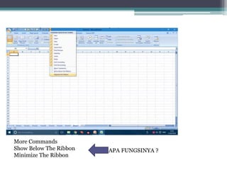
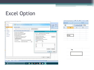
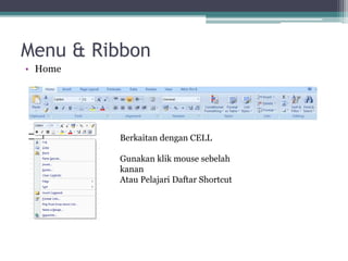
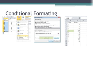
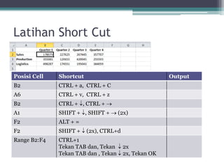
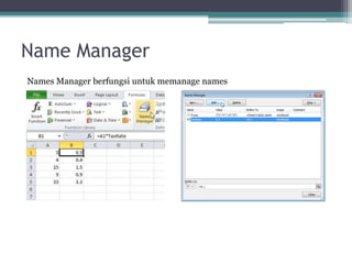
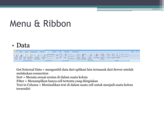
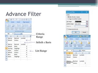
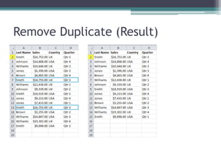
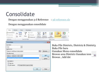
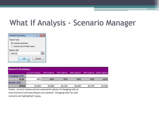
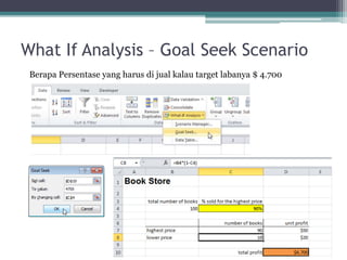
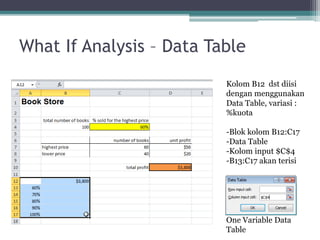
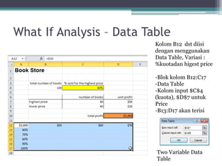
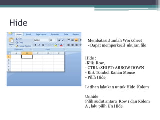
Microsoft Excel Training memberikan pelatihan mengenai penggunaan Microsoft Excel. Pelatihan ini membahas tentang fungsi-fungsi dasar Excel seperti penggunaan cells, format cells, conditional formatting, data validation, dan fungsi-fungsi dasar seperti matematika, statistik, dan tanggal. Pelatihan ini juga membahas cara membuat tabel, filter data, konsolidasi data, analisis 'what if', dan pembuatan pivot table.

1. Microsoft Excel Training
ِ
‫ر‬ْ‫ج‬َ‫أ‬ ُ‫ل‬ْ‫ث‬ِ‫م‬ ُ‫ه‬َ‫ل‬َ‫ف‬ ٍ
‫ْر‬‫ي‬َ‫خ‬ ‫ى‬َ‫ل‬َ‫ع‬ َّ‫ل‬َ‫د‬ ْ‫ن‬َ‫م‬
ِ‫ه‬ِ‫ل‬ِ‫ع‬‫ا‬َ‫ف‬
“Barangsiapa yang menunjuki kepada kebaikan maka dia akan
mendapatkan
pahala seperti pahala orang yang mengerjakannya.”

2. Time Frame
• 14 Mei 2016 – Fundamental excel
• 21 Mei 2016 – Best Practise For Business

3. Tujuan
• Familiar dengan penggunaan Excel
• Mengefisiensikan pekerjaan
• Mampu menjalankan excel dengan fungsi yang
optimal

4. MS Excel
• Microsoft Excel merupakan pesaing aplikasi
pengolahan data Lotus 123
• Secara umum Microsoft Excel memiliki 3 fungsi
:
▫ Database
▫ Pengolahan Angka
▫ Pembuatan Laporan

5. SPREADSHEET
A spreadsheet adalah suatu kertas kerja
untuk mengorganisasikan data dalam
baris dan kolom agar mudah untuk
membacanya dan
memanipulasi/mengolahnya.

6. Bagian dari Spread Sheet
1. Quick Access
ToolBar
2. Menu
3. Ribbon
4. Cell
5. Sheets
6. Column
7. Row
8. Formula Bar
9. Cell Reference
10. Splitting Spread sheet
11. Spreadsheet Grid
12. Zoom
13. Page Lay Out Button
14.Scroll Bar
15. Heading

7. Quick Access Tool Button
More Commands
Show Below The Ribbon
Minimize The Ribbon
APA FUNGSINYA ?

8. Office Button
Versi 2010 vs Versi 2007
Berbeda tampilan Icon , secara umum memiliki fungsi yang
sama sebagai “File Administration” (Pengelolaan File)

9. EXCEL OPTIONS
Perubahan berdampak
MS EXCEL yang diinstal di
komputer kita (kecuali
untuk advance)

10. Excel Option
R1 C1 Reference Cell

11. Excel Option

12. Excel Option

13. Excel Option

14. Excel Option

15. Excel Option

16. Excel Option

17. Excel Option

20. CELLS
• Cell
▫ Dapat digunakan untuk menginput data
▫ Data dapat diformat yang bemacam-macam : jenis, tampilan, posisi,
bentuk
• Jenis Data
▫ Numbers = nilai angka, dan dapat di jadikan bagian dalam kalkulasi
seperti + - / x
▫ Strings = adalah potongan kata, seperti : “AADC” , dapat dimanipulasi
dengan berbagai cara, seperti menemukan penggalan kata dalam
kalimat,
▫ Dates = mewakili hari dalam kalendar standar 5/19/2009
▫ Cell References = yaitu bagaimana excel di workbook.
▫ Fuctions = berupa rumus yang membuat kita menghitung secara cepat.
Sering sekali berdasarkan suatu content dari cell lainnya, dapat juga
menampilkan error seperti #N/A

21. Cell
Cell C3
Memilih 1
colom
Memilih 1 Row

22. CELL
Tekan CTRL
Tekan SHIFT
Disebut RANGE

23. Menu & Ribbon
• Home
Berkaitan dengan CELL
Gunakan klik mouse sebelah
kanan
Atau Pelajari Daftar Shortcut

24. Paste Special
1
2
4
5
3

25. Paste Special
• Paste
▫ All SEMUA, Content dan Format
▫ Formulas HANYA FORMULA > Lihat Formula Bar
▫ Values HANYA VALUE > lihat tampilan di Cell
▫ Formats HANYA FORMAT
▫ Comments HANYA COMMENT
▫ Validation VALIDATSI RULE >> DIBAHAS NANTI
▫ All using Source theme CONTENT DALAM
THEME.(VALUE + FORMAT)
▫ All except borders SEMUA, Kecuali Border
▫ Column widths HANYA MENGCOPY COLUMN WIDTH.
▫ Formulas and number formats HANYA FORMULA DAN
NUMBER FORMAT.
▫ Values and number formats HANYA VALUE DAN FORMAT

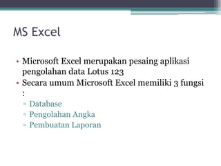
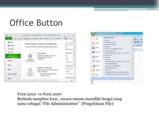
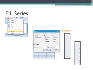
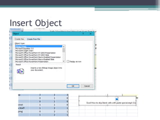
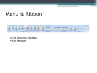
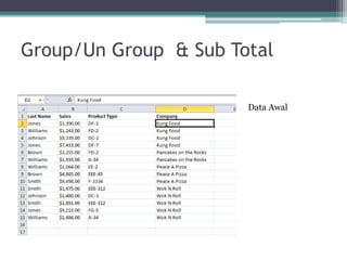
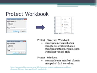
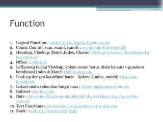
26. Paste Special
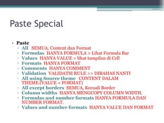
• Operation
▫ Specify which mathematical operation, if any, that you want to apply to the copied data.
▫ None TIDAK ADA OPERASI MATEMATIK DI DATA YANG DI COPIED
▫ Add / Substract / Multiply / Divide Data yang dicopy akan ditambahkan ke data di cel ataru range cell
yang dituju
▫ Skip blanks Excel How to skip blank cells with paste special.mp4
▫ Transpose Ubah kolom dari data yang di copy menjadi Baris, dan sebaliknya. Dengan menggunakan rumus
caranya :
Pilih area tujuan, ketik =transpose(array) lalu tekan CTRL+SHIFT+Enter. Catatan : Array = area baris
dan kolom yang akan di copy
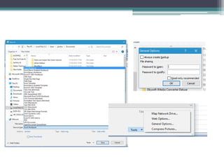
▫ Paste Link Linkk data = tampilan di formula Bar
▫ ='[namafile.xlsx]sheet’!CELL contoh = ‘[Bandung Lisna.xlsx]Bandung'!$C$143.

27. Insert Comment
Berfungsi untuk membuat
catatan Tambahan
Klik Mouse Kanan
Muncul :
Edit Comment
Delete Comment
Show/Hide Comment

28. Format Cell

29. Format Cell – Text &
• Wrap Text
Ukuran Font Tetap, Tinggi Kolom Diubah
• Shrink To Fit
Ukuran Font di kecilkan agar sesuai dengan Lebar Kolom
• Merge Cell
Lebih dari Satu Kolom atau lebih dari satu baris di satukan
• Locked Cell
akan berpengaruh pada saat sheet di proteksi, sehingga hanya cell yang unlocked yang bisa di
input/edit
• Hidden
akan berpengaruh pada saat sheet diproteksi, sehingga formula untuk cell tersebut
disembunyikan
• Tambah Baris dalam satu Cell
Gunakan ALT ENTER

30. Conditional Formating
Conditional Formating adalah suatu cara untuk menghighligt Cell tergantung
Nilai tertentu

31. Conditional Formating

32. Conditional Formating – Manage

33. Conditional Formating

34. Conditional Formating

35. Conditional Formating

36. Conditional Formating

37. Conditional Formating

38. Conditional Formating

39. Conditional Formating

40. Conditional Formating

41. Conditional Formating - compare

42. Conditional Formating

43. Conditional Formating

44. Conditional Formating + Developer

45. Conditional Formating

46. Format As a Table

47. Fill Range
Range adalah : Sekumpulan dua atau lebih Cell.
Fill Range : dapat dibuat dengan menklik sudut Cell, dan mengeser mouse ke
cell yang diinginkan (CLICK & DRAG)

48. Fill Range

49. Fill Series

50. Fill Justify
Befungsi merubah wrap
menjadi satu kata per baris

51. TABLES

52. Other
• Cell Style
• Insert
• Delete
• Format
• Sort & Filter
• Find and Select (Ctrl F / Ctrl H)

53. Latihan Short Cut
Posisi Cell Shortcut Output
B2 CTRL + a, CTRL + C
A6 CTRL + v, CTRL + z
B2 CTRL + , CTRL + 
A1 SHIFT + , SHIFT +  (2x)
F2 ALT + =
F2 SHIFT +  (2x), CTRL+d
Range B2:F4 CTRL+1
Tekan TAB dan, Tekan  2x
Tekan TAB dan , Tekan  2x, Tekan OK

54. Menu & Ribbon
• Insert
Insert Pivot akan dijelaskan nanti
Insert Tables = creatingtables
Insert Illustration ini jarang digunakan
Insert Chart akan dijelaskan nanti
Insert Link
Insert Text jarang digunakan
kecuali Header & Footer, Object

55. Insert Hyperlink

56. Insert Header & Footer
Page Layout Button

57. Insert Object

58. Menu & Ribbon
• Page Layout
Insert Themes, berguna untuk menentukan warna
tampilan, mirip seperti style. Namun dalam themes
setting dibuat untuk font, warna background, garis, dll

59. Page Setup
Options = Pengaturan Printer
Adjust to = biasanya excel menyesuaikan
otomatis, sehingga menjadi terlalu kecil
Fit to .... Pages width by .... Tall
= artinya melakukan adjustment, dengan
membagi sesuai lebar kertasnya.
Pengaturan Margin,
Center on Page = Menampilkan Worksheet
di tengah kertas sesuai batas margin

60. Page Setup

61. Menu & Ribbon
• Formulas
Berisi mengenai function
Name Manager

62. Status bar
Untuk memunculkan hal-hal khusus ,
Klik Mouse Kanan di status Bar

63. Names
Membuat Names untuk cell atau
rannge bisa dengan 3 cara :
1. Icon Define Names
2. Names Manager
3. Klik Mouse Kanan, pilih Name
Rage

64. Names
Names adalah salah satu cara untuk mempermudah membuat formula,
Names diberikan kepada cell atau range of cell
Ketik di cell A 5
=Sum(Prices)
Ketik di Cell B1
=A1*TaxRate

65. Name Manager
Names Manager berfungsi untuk memanage names

66. Beda Formula dengan Function
Formula Function

67. Formula & Function
• Lookup Function
• Logical Function
• Mathematical Function
• Statistical Function
• String Function
• Date & Time
• Text
• dll

68. Cara Mendefinisikan Function
Formula terdiri dari : satu atau beberapa function. Setiap Function
dibuat dari tiga komponen
1. Function Name , contoh SUM, Average
2. Arguments, adalah susunan kalimat dari Function tersebut
3. Output, adalah hasil dari function ketika selesai melakukan kalkulasi.
Contoh :

69. Menu & Ribbon
• Data
Get External Data = mengambil data dari aplikasi lain termasuk dari Server setelah
melakukan connection
Sort = Menata sesuai urutan di dalam suatu kolom
Filter = Menampilkan hanya cell tertentu yang diinginkan
Text to Column = Memisahkan text di dalam suatu cell untuk menjadi suatu kolom
tersendiri

70. From Text

71. Sort
Fungsi : Mengurutkan, coba dengan file berikut
Cara 1, One Column
Cara 2, Multiple Column

72. Filter
Pilih Count USA
Pilih Quarter Q4

73. Advance Filter
Criteria
Range
List Range
Selisih 1 Baris

74. Advance Filter
Latihan (Clear filter setiap memulai)
• Tulis Biru di Cell A3, Lakukan
Advance Filter, catat hasilnya
• Tulis Kubus di Cell B3, Lakukan
Advance Filter, catat hasilnya
• Ganti Tuliskan Kubus di Cell B3
dengan Bola, Lakukan Advance
Filter, Catat Hasilnya.

75. Text To Column

76. Remove Duplicate

77. Remove Duplicate (Result)

78. Remove Duplicate (2)

79. Remove Duplicate (Result 2)

80. Data Validation
Teknik Input Data untuk meminimalisasi kesalahan typho,
dengan cara membuat batasan tertentu untuk mengiput data ke
suatu cell
• Any Value = Tidak ada batasan
• Whole Number
• Decimal
• List
• Date
• Time
• Text length
• Custom

81. Data Validation – Whole Number
Tuliskan di Cell B2
Berapa Kali Anda Sholat dalam sehari ?
Sheet Input Message :
Title : Jumlah Sholat
Input Message :
Isi dengan Angka 0 sampai 10
Sheet Error Allert :
STYLES : STOP
TITLE : Lebih Dari Batasan
ERROR MESSAGE : Alim Banget

82. Data Validation – Decimal
Blok Range C2:C10
Coba Input angka di area
23 di Cell C2 >> Keluar
warning
Coba Input angka 4 di cel
A10
Beda dengan whole
number, pada whole
number tidak bisa dibuat
value decimal

83. Data Validation – List
Buat di Sheet 1 :
Name Range Address
Food A1:A3
Pizza B1:B4
Pancakes C1:C2
Chinese D1:D3
Buat di Sheet 2 :
Berikan Nama Range:

84. Data Validation - List

85. Data Validation – Date

86. Data Validation – Text length
c
Coba Input nama “Maya”
di Cell B1
Coba Input nama
Herman Syahroni di Celll
B2

87. Data Validation – Custom
Block Range A2 : A20
Coba Input angka di area
cell A2 s/d A 5 = 1,2,3
Coba Input angka 3 di cel
A10 >> Keluar warning

88. Circle Invalid Data
1. Cell A1, Buat Formula =RandBetween(300;500)
2. Copy A1 ke Range A1 s/d Q20
3. Blok Range A1 s/d Q 20
4. Buat Data Validation, Whole Number, Between 350:450
5. Click CIRCLE INVALID DATA > Lihat Hasilnya

89. Consolidate
Dengan menggunakan 3 d Reference : 3d-reference.xls
Dengan menggunakan consolidate
Buka File District1, District2 & District3
Buka File baru
Gunakan Menu consolidate
Browse area District1 Gunakan icon
Browse , Add dst

90. What if Analysis
Scenario Manager
Asumsikan stock toko buku = 100 buah
Sejumlah X di jual dengan dengan profit $ 50
Sejumlah Y di jual dengan profit $ 20
X dan Y di hitung dengan proporsi tertentu dari Jumlah Buku

91. What if Analysis – Scenario Manager
Bagaimana kalau 50 %, 60 %, 70 %, 80 % dan 100 %
Alternatif 1 = coba sendiri
Alternatif 2 = scenario manager

92. What If Analysis - Scenario Manager

93. What If Analysis - Scenario Manager

94. What If Analysis – Goal Seek Scenario
Berapa Persentase yang harus di jual kalau target labanya $ 4.700

95. What If Analysis – Data Table
Kolom B12 dst diisi
dengan menggunakan
Data Table, variasi :
%kuota
-Blok kolom B12:C17
-Data Table
-Kolom input $C$4
-B13:C17 akan terisi
One Variable Data
Table

96. What If Analysis – Data Table
Kolom B12 dst diisi
dengan menggunakan
Data Table, Variasi :
%kuotadan higest price
-Blok kolom B12:C17
-Data Table
-Kolom input $C$4
(kuota), $D$7 untuk
Price
-B13:D17 akan terisi
Two Variable Data
Table

97. Group/Un Group & Sub Total
Data Awal

98. Group/Un Group & Sub Total

99. Group/Un Group & Sub Total
Pilih kolom A dan B,
lakukan grouping

100. Menu & Ribbon
• Review
Protect Sheet = berkaitan dengan Lock/Unlock Cell
Bila diprotect worksheet, user tidak dapat
melakukan perubahan seperti insert, modify,
delete, atau format data.
Action yang akan di protect harus di centang

101. Protect Workbook
Protect : Structure Workbook
= mencegah menambah atau
menghapus worksheet, atau
mencegah untuk menampilkkan
worksheet yang di Hide
Protect : Windows
= mencegah user merubah ukuran
atau poisisi dari worksheet
https://support.office.com/en-us/article/Password-protect-worksheet-or-workbook-
elements-dbf706e0-ba22-4a08-84d8-552db16eef11

102. Share workbook
Kita dapat bekerja dengan orang lain di workbook yang sama pada saat yang sama.
- Workbook harus di save di network dimana orang lain dapat membuka file tersebut.
- Sebaiknya di pasangkan track of change

103. Share workbook

104. Menu & Ribbon
• View
Split = Layar Worksheet dibagi dua atau empat
Freezepane = Salah satu bagian worksheet ada yang di freeze
(tetap dan tidak bergerak)

105. Hide
Membatasi Jumlah Worksheet
- Dapat memperkecil ukuran file
Hide :
-Klik Row,
- CTRL+SHIFT+ARROW DOWN
- Klik Tombol Kanan Mouse
- Pilih Hide
Latihan lakukan untuk Hide Kolom
Unhide
Pilih sudut antara Row 1 dan Kolom
A , lalu pilih Un Hide

106. Pivot
Digunakan untuk membuat ekstrasi informasi dari sekumpulan data tables
Persyaratan :
1. Ada SOURCE DATA dalam bentuk TABULAR dengan HEADER
2. HEADER terdiri dari 1 ROW,
3. TIDAK ADA BLANK ROW, BLANK COLUMN & MERGE CELL

107. PIVOT

109. Graphics

110. Chart
Pareto Chart
1. Gunakan Bar Chart
2. Klik Kanan, pada
redbare, dan pilih
Change series chart type
menjadi Line with
Marker
3. Klik kanan garis merah
dengan format data
series

113. Function
1. Logical Function : nested-if.xls, logical-functions.xls
2. Count, Countif, sum, sumif, sumifs : count-sum-functions.xls
3. Hlookup, Vlookup, Match,Index, Choose : lookup-reference-functions.xls;
tax-rates.xls
4. Offset : offset.xls
5. LeftLooup (kalau Vlookup, kolom acuan harus disisi kanan) > gunakan
kombinasi Index & Match : left-lookup.xls
6. Look up dengan koordinat baris – kolom (Index, match) : two-way-
lookup.xls
7. Lokasi suatu value dan fungsi max : locate-maximum-value.xls
8. Indirect : indirect.xls
9. Date : date-time-functions.xls, datedif.xls, weekdays.xls, day-of-the-
year.xls
10. Text Functions text-functions.xls; number-of-words.xlsx
11. Rank : rank.xls, forecast-trend.xls

114. Error
The #NAME? error occurs when Excel does
not recognize text in a formula.
##### error
When your cell contains this error code,
the column isn't wide enough to display the
valu
Excel displays the #VALUE! error when a
formula has the wrong type of argument.

115. Error (2)
Excel displays the #DIV/0! error when a
formula tries to divide a number by 0 or an
empty cell.
Excel displays the #REF! error when a
formula refers to a cell that is not valid.

116. Merge with Words
• Siapkan file words
• Siapkan file excel
• Desain isi tabel di excel, sesuaikan dengan field di
words
▫ Buat minimal 1 baris data
• Buka mailing merge di words
▫ Mailing
▫ Start Mail Merge > Letter
▫ Select Recipient > Use Existing List (pilih file
excelnya)
▫ Insert Mergefile ke file words
▫ Save file words

117. ‫ا‬ِ‫ب‬ َ‫ون‬ُ‫ر‬ُ‫م‬ْ‫أ‬َ‫ت‬ ِ‫اس‬َّ‫ن‬‫ل‬ِ‫ل‬ ْ‫َت‬‫ج‬ِ‫ر‬ْ‫خ‬
ُ
‫أ‬ ٍ‫ة‬َّ‫م‬
ُ
‫أ‬ َ‫ر‬ْ‫ي‬َ‫خ‬ ْ‫م‬ُ‫ت‬ْ‫ن‬ُ‫ك‬
َ‫ك‬ْ‫ن‬ُ‫م‬ْ‫ال‬ ِ‫ن‬َ‫ع‬ َ‫ن‬ْ‫و‬َ‫ه‬ْ‫ن‬َ‫ت‬َ‫و‬ ِ‫ف‬‫و‬ُ‫ر‬ْ‫َع‬‫م‬ْ‫ل‬
ِ‫ر‬
”Kamu adalah umat yang terbaik yang dilahirkan untuk
manusia, menyuruh kepada yang ma’ruf, dan mencegah
dari yang munkar.” (QS. Ali Imran: 110).