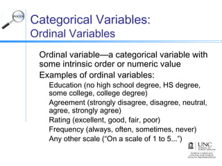
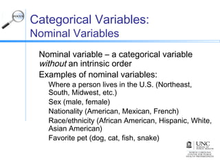
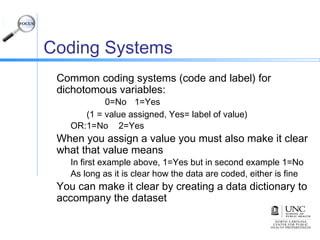
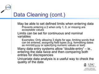
This document discusses the basics of descriptive data analysis, including defining different types of variables, coding principles, and univariate data analysis. It describes continuous variables as always numeric and categorical variables as information sorted into categories, with ordinal variables having intrinsic order, nominal variables lacking order, and dichotomous variables having only two levels. The document outlines steps for coding variables and cleaning data, as well as techniques for univariate analysis of continuous and categorical variables to check data quality.

1. Data Analysis Basics:
Variables and Distribution

2. Goals
Describe the steps of descriptive data
analysis
Be able to define variables
Understand basic coding principles
Learn simple univariate data analysis

3. Types of Variables
Continuous variables:
Always numeric
Can be any number, positive or negative
Examples: age in years, weight, blood pressure
readings, temperature, concentrations of
pollutants and other measurements
Categorical variables:
Information that can be sorted into categories
Types of categorical variables – ordinal, nominal
and dichotomous (binary)

4. Categorical Variables:
Ordinal Variables
Ordinal variable—a categorical variable with
some intrinsic order or numeric value
Examples of ordinal variables:
Education (no high school degree, HS degree,
some college, college degree)
Agreement (strongly disagree, disagree, neutral,
agree, strongly agree)
Rating (excellent, good, fair, poor)
Frequency (always, often, sometimes, never)
Any other scale (“On a scale of 1 to 5...”)

5. Categorical Variables:
Nominal Variables
Nominal variable – a categorical variable
without an intrinsic order
Examples of nominal variables:
Where a person lives in the U.S. (Northeast,
South, Midwest, etc.)
Sex (male, female)
Nationality (American, Mexican, French)
Race/ethnicity (African American, Hispanic, White,
Asian American)
Favorite pet (dog, cat, fish, snake)

6. Categorical Variables:
Dichotomous Variables
Dichotomous (or binary) variables – a
categorical variable with only 2 levels of
categories
Often represents the answer to a yes or no
question
For example:
“Did you attend the church picnic on May 24?”
“Did you eat potato salad at the picnic?”
Anything with only 2 categories

7. Coding
Coding – process of translating information
gathered from questionnaires or other
sources into something that can be analyzed
Involves assigning a value to the information
given—often value is given a label
Coding can make data more consistent:
Example: Question = Sex
Answers = Male, Female, M, or F
Coding will avoid such inconsistencies

8. Coding Systems
Common coding systems (code and label) for
dichotomous variables:
0=No 1=Yes
(1 = value assigned, Yes= label of value)
OR:1=No 2=Yes
When you assign a value you must also make it clear
what that value means
In first example above, 1=Yes but in second example 1=No
As long as it is clear how the data are coded, either is fine
You can make it clear by creating a data dictionary to
accompany the dataset

9. Coding: Dummy Variables
A “dummy” variable is any variable that is coded to
have 2 levels (yes/no, male/female, etc.)
Dummy variables may be used to represent more
complicated variables
Example: # of cigarettes smoked per week--answers total 75
different responses ranging from 0 cigarettes to 3 packs per
week
Can be recoded as a dummy variable:
1=smokes (at all) 0=non-smoker
This type of coding is useful in later stages of
analysis

10. Coding:
Attaching Labels to Values
Many analysis software packages allow you to attach a
label to the variable values
Example: Label 0’s as male and 1’s as female
Makes reading data output easier:
Without label: Variable SEX Frequency Percent
0 21 60%
1 14 40%
With label:Variable SEX Frequency Percent
Male 21 60%
Female 14 40%

11. Coding- Ordinal Variables
Coding process is similar with other categorical
variables
Example: variable EDUCATION, possible coding:
0 = Did not graduate from high school
1 = High school graduate
2 = Some college or post-high school education
3 = College graduate
Could be coded in reverse order (0=college graduate,
3=did not graduate high school)
For this ordinal categorical variable we want to be
consistent with numbering because the value of the
code assigned has significance

12. Coding – Ordinal Variables
(cont.)
Example of bad coding:
0 = Some college or post-high school education
1 = High school graduate
2 = College graduate
3 = Did not graduate from high school
Data has an inherent order but coding does
not follow that order—NOT appropriate
coding for an ordinal categorical variable

13. Coding: Nominal Variables
For coding nominal variables, order makes no
difference
Example: variable RESIDE
1 = Northeast
2 = South
3 = Northwest
4 = Midwest
5 = Southwest
Order does not matter, no ordered value
associated with each response

14. Coding: Continuous Variables
Creating categories from a continuous variable (ex.
age) is common
May break down a continuous variable into chosen
categories by creating an ordinal categorical variable
Example: variable = AGECAT
1 = 0–9 years old
2 = 10–19 years old
3 = 20–39 years old
4 = 40–59 years old
5 = 60 years or older

15. Coding:
Continuous Variables (cont.)
May need to code responses from fill-in-the-blank
and open-ended questions
Example: “Why did you choose not to see a doctor about
this illness?”
One approach is to group together responses with
similar themes
Example: “didn’t feel sick enough to see a doctor”,
“symptoms stopped,” and “illness didn’t last very long”
Could all be grouped together as “illness was not severe”
Also need to code for “don’t know” responses”
Typically, “don’t know” is coded as 9

16. Coding Tip
Though you do not code until the data
is gathered, you should think about how
you are going to code while designing
your questionnaire, before you gather
any data. This will help you to collect
the data in a format you can use.

17. Data Cleaning
One of the first steps in analyzing data is to
“clean” it of any obvious data entry errors:
Outliers? (really high or low numbers)
Example: Age = 110 (really 10 or 11?)
Value entered that doesn’t exist for variable?
Example: 2 entered where 1=male, 0=female
Missing values?
Did the person not give an answer? Was answer
accidentally not entered into the database?

18. Data Cleaning (cont.)
May be able to set defined limits when entering data
Prevents entering a 2 when only 1, 0, or missing are
acceptable values
Limits can be set for continuous and nominal
variables
Examples: Only allowing 3 digits for age, limiting words that
can be entered, assigning field types (e.g. formatting dates
as mm/dd/yyyy or specifying numeric values or text)
Many data entry systems allow “double-entry” – ie.,
entering the data twice and then comparing both
entries for discrepancies
Univariate data analysis is a useful way to check the
quality of the data

19. Univariate Data Analysis
Univariate data analysis-explores each
variable in a data set separately
Serves as a good method to check the quality of
the data
Inconsistencies or unexpected results should be
investigated using the original data as the
reference point
Frequencies can tell you if many study
participants share a characteristic of interest
(age, gender, etc.)
Graphs and tables can be helpful

20. Univariate Data Analysis (cont.)
Examining continuous variables can give you
important information:
Do all subjects have data, or are values missing?
Are most values clumped together, or is there a lot
of variation?
Are there outliers?
Do the minimum and maximum values make
sense, or could there be mistakes in the coding?

21. Univariate Data Analysis (cont.)
Commonly used statistics with univariate
analysis of continuous variables:
Mean – average of all values of this variable in
the dataset
Median – the middle of the distribution, the
number where half of the values are above and
half are below
Mode – the value that occurs the most times
Range of values – from minimum value to
maximum value

22. Statistics describing a continuous
variable distribution
84 = Maximum (an
outlier)
2 = Minimum
28 = Mode (Occurs
twice)
33 = Mean
36 = Median (50th
Percentile)

23. Standard Deviation
Figure left: narrowly distributed age values (SD = 7.6)
Figure right: widely distributed age values (SD = 20.4)

24. Distribution and Percentiles
Distribution –
whether most values
occur low in the
range, high in the
range, or grouped in
the middle
Percentiles – the
percent of the
distribution that is
equal to or below a
certain value
Distribution curves for variable AGE
25th Percentile
(4 years)
25th Percentile
(6 years)

25. Analysis of Categorical Data
Distribution of
categorical variables
should be examined
before more in-
depth analyses
Example: variable
RESIDE
Number of people answering example questionnaire who reside in 5
regions of the United States

26. Analysis of Categorical Data (cont.)
Another way to look
at the data is to list
the data categories
in tables
Table shown gives
same information as
in previous figure
but in a different
format
Frequency Percent
Midwest 16 20%
Northeast 13 16%
Northwest 19 24%
South 24 30%
Southwest 8 10%
Total 80 100%
Table: Number of people answering sample
questionnaire who reside in 5 regions of the United
States

27. Observed vs. Expected Distribution
Education variable
Observed distribution of
education levels (top)
Expected distribution of
education (bottom) (1)
Comparing graphs shows a
more educated study
population than expected
Are the observed data really
that different from the
expected data?
Answer would require further
exploration with statistical
tests
Observed data on level of education from a hypothetical
questionnaire
Data on the education level of the US population aged 20
years or older, from the US Census Bureau

28. Conclusion
Defining variables and basic coding are
basic steps in data analysis
Simple univariate analysis may be used
with continuous and categorical
variables
Further analysis may require statistical
tests such as chi-squares and other
more extensive data analysis

29. References
1. US Census Bureau. Educational Attainment in the
United States: 2003---Detailed Tables for Current
Population Report, P20-550 (All Races). Available at:
http://www.census.gov/population/www/socdemo/educa
. Accessed December 11, 2006.