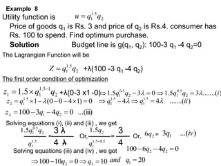
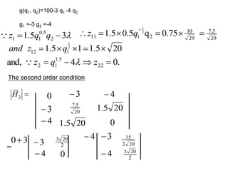
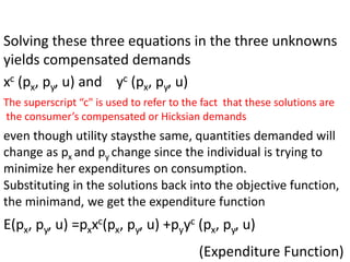
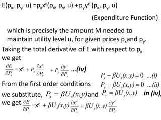
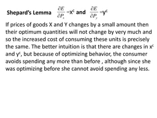
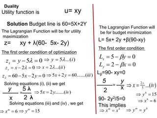
The document outlines the mathematical economics principles related to consumer behavior, focusing on utility maximization under budget constraints and key concepts such as the Slutsky equation, substitution and income effects. It discusses the Lagrange function for maximizing utility, along with necessary conditions for equilibrium and convexity of indifference curves. Additionally, it presents mathematical formulations guiding consumer choice and the decomposition of price effects into substitution and income effects.

![
d
dy
dx
or,
33
23
13
32
22
12
31
21
11
1
C
C
C
C
C
C
C
C
C
A
y
x
y
x
ydp
xdP
dM
dp
dp
So,
A
dx
1
11
[ C
dPx
21
C
dPy
]
)
( 31
C
ydp
xdP
dM y
x
A
dy
1
12
[ C
dPx
22
C
dPy
]
)
( 32
C
ydp
xdP
dM y
x
A
d
1
13
[ C
dPx
23
C
dPy
]
)
( 33
C
ydp
xdP
dM y
x
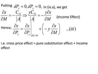
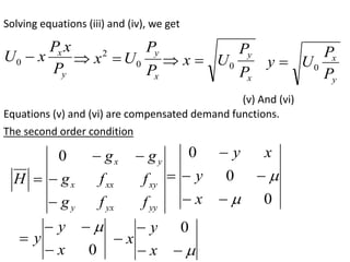
…(ix a)
…(ix b)
…(ix c)
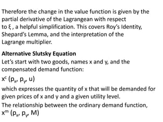
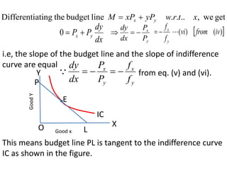
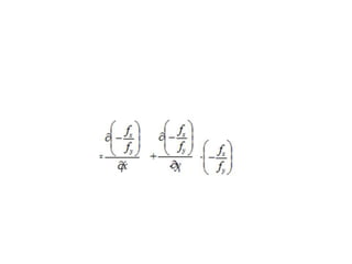
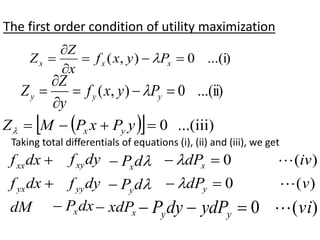
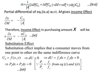
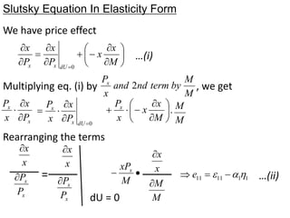
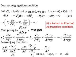
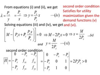
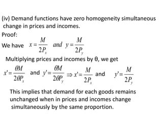
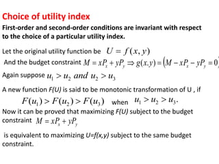
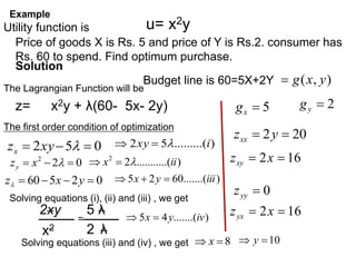
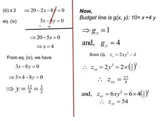
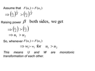
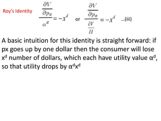
Consumer's equilibrium can change with the change
in income, prices, and relative prices. In order to find
the effect of change in price or income, all variables
are allowed to vary simultaneously.](https://image.slidesharecdn.com/mathematicaleconomicsunit1-231105151144-851fcf68/85/Mathematical-Economics-unit-1-pptx-16-320.jpg)
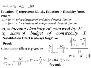
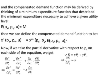
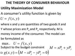
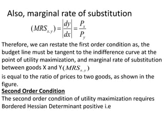
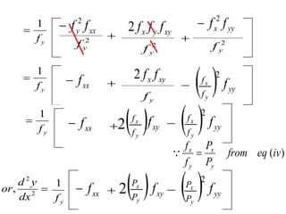
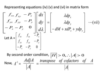
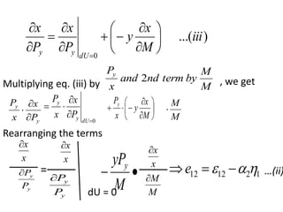
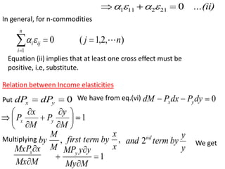
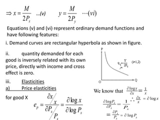
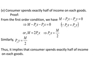
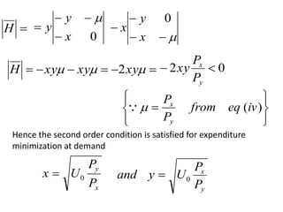
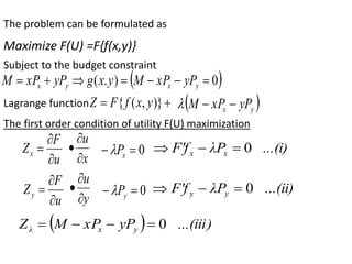
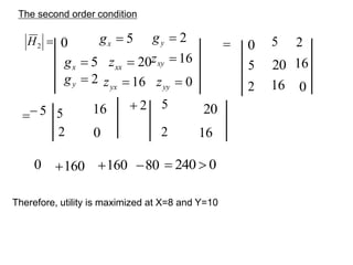
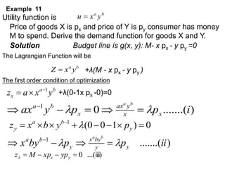
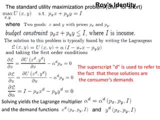
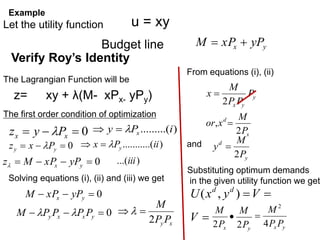
![Interpretation of Lagrange Multiplier
We have utility function )
,
( y
x
f
U
Diff. w.r.t.M, we get
M
U
M
x
fx
M
y
fy
Substituting y
y
x
x P
f
and
P
f
)
(
&
)
( ii
i
eq
from s
We get
M
U
M
x
Px
M
y
Py
M
U
or,
M
x
Px
[
]
M
y
Py
…(a)
We have budget line y
x yP
xP
M
M
M
1
M
y
P
M
x
P y
x
…(b)
Therefore, from (a) and (b),
M
U
= marginal utility of money.](https://image.slidesharecdn.com/mathematicaleconomicsunit1-231105151144-851fcf68/85/Mathematical-Economics-unit-1-pptx-24-320.jpg)
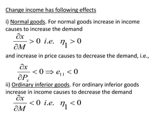
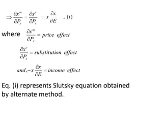
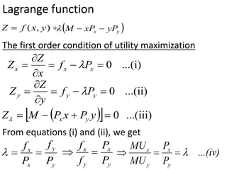
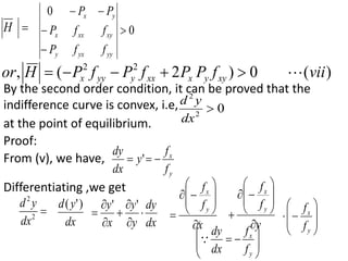
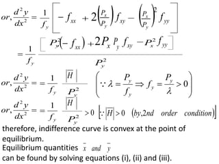
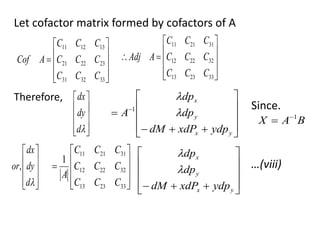
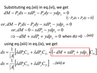
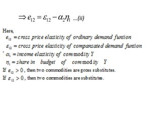
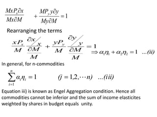
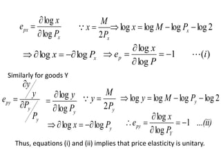
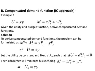
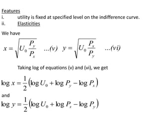
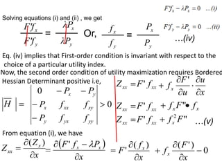
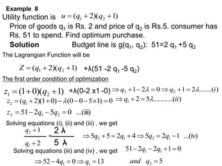
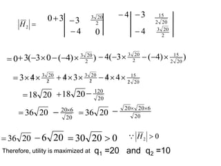
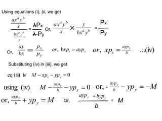
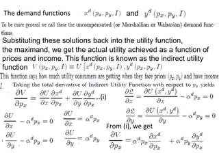
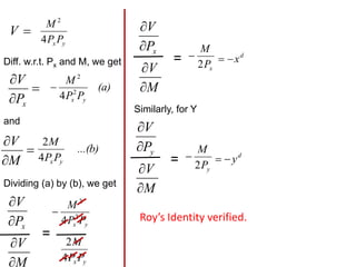
![Cross Effect
Cross effect deals with the effect of change in price of one
commodity on the demand for other commodity.
To find the effect of a change in price Py of goods Y on quantity ,
we keep price Px and money income M constant so
,
0
,
0
dM
dPx
From eq. (ix.a), we get
A
dx
1
11
[ C
dPx
21
C
dPy
]
)
( 31
C
ydp
xdP
dM y
x
…(ix a)
A
yC
A
C
P
x
y
31
21
,
0
,
0
since,
dM
dPx
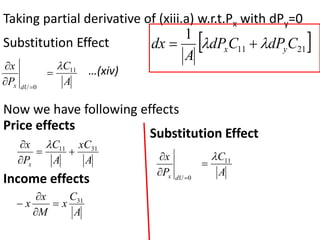
(Price Effect)
when and
dU 0
0
y
x ydp
xdP
dM
we get from (ix.a)
A
C
P
x
y
21
(Substitution Effect)
(Substitution Effect)](https://image.slidesharecdn.com/mathematicaleconomicsunit1-231105151144-851fcf68/85/Mathematical-Economics-unit-1-pptx-27-320.jpg)
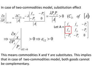


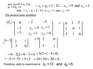

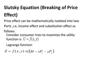
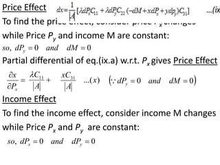
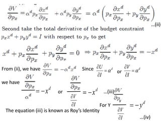
![Or, y
ayp y
byp
= bM Or, b]
[a
ypy = bM
y
=
Mb
b]
[a
py
Now using (iv)
b
ayp
x
y
xp y
or,
x
y
bp
ap
x
or, x
y
p
b
p
a
x
x
Mb
b]
[a
py
or, )
( b
a
p
Ma
x
x
….(v)
….(vi)
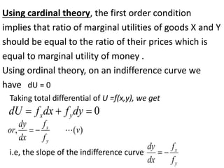
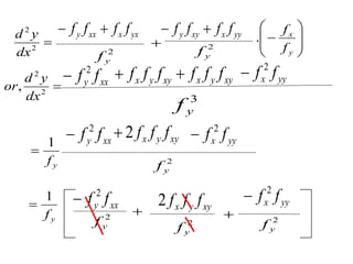
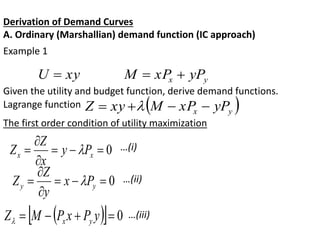
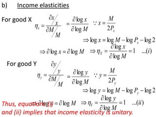
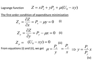
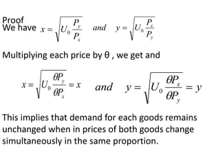
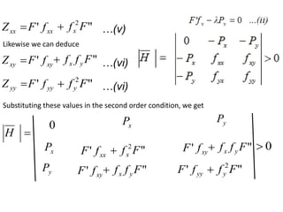
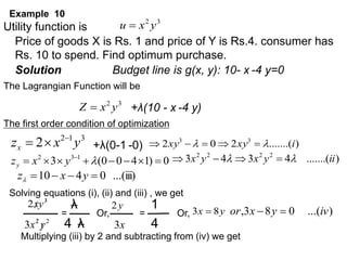
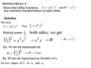
Equations (v) and (vi) represent demand function for goods Y and X
Respectively.](https://image.slidesharecdn.com/mathematicaleconomicsunit1-231105151144-851fcf68/85/Mathematical-Economics-unit-1-pptx-70-320.jpg)


![Or, y
ayp y
byp
= bM Or, b]
[a
ypy = bM
y
=
Mb
b]
[a
py
Now using (iv)
b
ayp
x
y
xp y
or,
x
y
bp
ap
x
or, x
y
p
b
p
a
x
x
Mb
b]
[a
py
or, )
( b
a
p
Ma
x
x
….(v)
….(vi)
Equations (v) and (vi) represent demand function for goods Y and X
Respectively.](https://image.slidesharecdn.com/mathematicaleconomicsunit1-231105151144-851fcf68/85/Mathematical-Economics-unit-1-pptx-73-320.jpg)
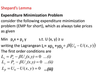
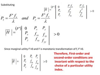
![
x
P
E
xc (x,y)
βUx
x
c
P
x
(x,y)
βUy
x
c
P
y
x
P
E
xc (x,y)
U
β x
[
x
c
P
x
(x,y)
Uy
]
x
c
P
y
…(v)
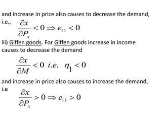
we differentiate the constraint U (xc, Yc) = u totally
with respect to px to get
x
U
x
c
P
x
y
U
x
c
P
y
= 0 Since utility u is fixed.
So from (v), we get
x
P
E
xc …(vi)
Similarly, taking the total derivative of E with
respect to py we get
y
P
E
yc …(vii)
The results (vi) and (vii) are known as Shepard’s Lemma](https://image.slidesharecdn.com/mathematicaleconomicsunit1-231105151144-851fcf68/85/Mathematical-Economics-unit-1-pptx-85-320.jpg)
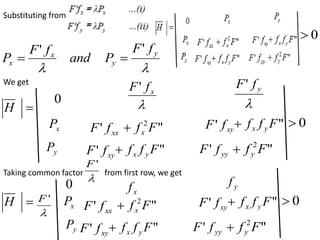
![for which the first two first order conditions are given
by
x
L
x
y
x
f )
,
,
(
...(ii)
x
)
g(x,y
λ 0
,
y
L
y
y
x
f )
,
,
(
)
...(iii
y
)
g(x,y
λ 0
,
Let optimum values be x* and y*
Substituting the solutions into the function f gives the
value function
)
(
F .(iv)
ξ),ξ] ..
y
(
f[x *
*
(
),
which is the maximized value of f , which ultimately
depends on ξ. Taking the total derivative of F (ξ) we
get](https://image.slidesharecdn.com/mathematicaleconomicsunit1-231105151144-851fcf68/85/Mathematical-Economics-unit-1-pptx-89-320.jpg)
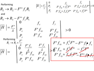
![
)
(
F ]
),
(
),
(
[ *
*
y
x
f
)
(
F
x
f
d
dx*
y
f
d
dy*
...(v)
ξ
f
The last term represents the direct effect of ξ on f , while the
first two terms represent the indirect effect of ξ on f by
changing x∗ and y∗. This expression can be simplified in two
steps. First substituting in the first order conditions
∂f /∂x = λ∂g/∂x and ∂f /∂y = λ∂g/∂y into (v) gives
x
y
x
f )
,
,
(
0
x
g(x,y,ξ(
λ
y
y
x
f )
,
,
(
0
y
g(x,y,ξ(
λ
)
(
F
x
g
*
d
dx*
y
g
*
d
dy*
ξ
f
](https://image.slidesharecdn.com/mathematicaleconomicsunit1-231105151144-851fcf68/85/Mathematical-Economics-unit-1-pptx-90-320.jpg)
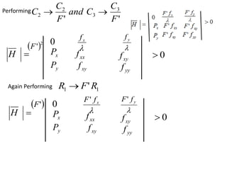
![
)
(
F
x
g
*
d
dx*
y
g
*
d
dy*
ξ
f
)
(
,
F
or
x
g
[
*
d
dx*
y
g
]
*
d
dy
...(vi)
ξ
f
Second, differentiating the constraint g (x∗, y∗, ξ) = c totally
with respect to ξ gives
x
g
d
dx*
y
g
0
*
g
d
dy
x
g
d
dx*
y
g
g
d
dy*
which substituting into (vi) and rearranging gives the envelope theorem
)
(
F
ξ
f
g
*
ξ
L
(Envelope Theorem)](https://image.slidesharecdn.com/mathematicaleconomicsunit1-231105151144-851fcf68/85/Mathematical-Economics-unit-1-pptx-91-320.jpg)