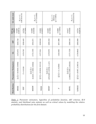
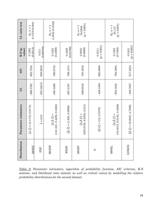
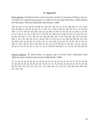
1. The document describes fitting several Marshall-Olkin distributions (MOEE, MOEW, MOEP, MOEL) as well as exponential, Weibull, Pareto and Lomax distributions to two real datasets using maximum likelihood estimation in R. For each distribution, it provides the cumulative distribution function, probability distribution function, likelihood function, and maximum likelihood estimates. It performs Kolmogorov-Smirnov goodness of fit tests to compare the fitted distributions to the datasets. 2. Functions for the cumulative distribution function, probability distribution function, and likelihood function are provided for each of the MOEE, MOEW, MOEP, MOEL and MOELFR distributions. Maximum likelihood estimation and Kolmogorov-Sm

1. 1
Marshall – Olkin distributions in R
Achilleas Papatsimpas
M.Sc. Statistics and Operational Research
The fit of the generalized MOEE, MOEW, MOEP and MOEL distributions which is
presented in Chapter 4 of my M.Sc. Thesis “Univariate Marshall – Olkin
distributions: A critical review” is applied in two real datasets. The first dataset
consists of 213 observations concerning the number of successive failures of every
aircraft’s air conditioning system from a fleet of 13 aircrafts (Proschan, 1963;
Dahiya and Gurland, 1972 and Adamidis and Loukas, 1998). The second dataset
consists of 72 observations of guinea pigs’ survival times inoculated with different
doses of tuberculosis bacteria (Bjerkedal, 1960).
MOEE, MOEW, MOEP, MOEL, EXP, WEIB, P and LOMAX distributions were
fitted to this data using the R programming language.
For each of the above distributions, unknown parameters were estimated by using
the maximum likelihood method, while calculating the maximum likelihood
estimators, the Kolmogorov-Smirnov (K-S) test was used to test the adaptability of
each distribution. The estimators, the logarithm of the likelihood function (LL), the
AIC (Akaike Information Criterion) criterion, the value of the KS test statistic and
the corresponding p-value of the hypothesis test that if it is necessary to add a new
parameter in the initial distribution is given in Tables 1 and 2. The AIC criterion,
introduced in the literature by Akaike (1969), is calculated from the relation
2 2AIC k LL  where k is the number of the unknown parameters of the model.
Considering the model selection, the preferred model is the one with the lowest AIC
value.
1. Marshall-Olkin Extended Exponential distribution (MOEE)
Cumulative distribution function
 
1
; , ,
1
x
x
e
G x a
e a





 
cdfmoee<-function(x,a,l){

2. 2
cdf=(exp(l*x)-1)/(exp(l*x)-1+a)
return(cdf)
}
Probability distribution function
 
 
2
; , ,
1 (1 )
x
x
a e
g x a
a e







 
pdfmoee<-function(x,a,l){
pdf=(a*l*exp(-l*x))/(1-(1-a)*exp(-l*x))^2
return(pdf)
}
Logarithm of the Likelihood function
       
1 1
log ; ; log 2 log 1 (1 ) .i
n n
t
obs obs i
i i
L y l y n a t a e 
    
 
      
llmoee<-function(a,l){
x=dataset
n=length(x)
-n*log(a*l)+l*sum(x)+2*sum(log(1-(1-a)*exp(-l*x)))
}
Maximum likelihood estimators
est<-mle(minuslog=llmoee, start=list(a=0.5849, l=0.0082))
summary(est)
Kolmogorov-Smirnov test
ks.test(dataset, cdfmoee, a=0.5849, l=0.0082)

3. 3
2. Marshall-Olkin Extended Weibull distribution (MOEW)
Cumulative distribution function
 
 
 
1
; , , ,
1 (1 )
x
x
e
G x a
a e




 




 
cdfmoew<-function(x,a,b,l){
cdf=(1-exp(-(l*x)^b))/(1-(1-a)*exp(-(l*x)^b))
return(cdf)
}
Probability distribution function
 
   
 
1
2
; , , ,
1 (1 )
x
x
a x e
g x a
a e


 

 
 
 


    
pdfmoew<-function(x,a,b,l){
pdf=(a*b*l*(l*x)^(b-1)*exp(-(l*x)^b))/(1-(1-a)*exp(-(l*x)^b))^2
return(pdf)
}
Logarithm of the Likelihood function
         
1 1
log ; ; log 1 log
n n
obs obs i i
i i
L y l y n a t t  
    
 
     
 
 1
2 log 1 (1 ) .i
n
t
i
a e



  
llmoew<-function(a,b,l){
x=dataset
n=length(x)
-n*log(a)-n*log(b)-n*b*log(l)-(b-1)*sum(log(x))+l^b*sum(x^b)+2*sum(log(1-(1-a)*exp(-
(l*x)^b)))
}
Maximum likelihood estimators
est<-mle(minuslog=llmoew, start=list(a=0.2531, b=1.1905, l=0.0052))

4. 4
summary(est)
Kolmogorov-Smirnov test
ks.test(dataset, cdfmoew, a=0.2531, b=1.1905, l=0.0052)
3. Marshall-Olkin Extended Pareto distribution (MOEP)
Cumulative distribution function
 ; , ,
1
,
1
x
x
a
G x a


 


 
 
 
 
  
 
cdfmoep<-function(x,a,b,l){
cdf=((x^l/b^l)-1)/((x^l/b^l)-1+a)
return(cdf)
}
Probability distribution function
1
2
( ; , , ) ,
1
x
a
g x a
x
a



 



 
 
 
  
   
   
pdfmoep<-function(x,a,b,l){
pdf=(a*l*(x^(l-1)/b^(l-1)))/(b*((x^l/b^l)-1+a)^2)
return(pdf)
}

5. 5
Logarithm of the Likelihood function
   
1
log ; ; log ( 1)log 2log 1 .
n
i i
obs obs
i
t ta
L y l y n a


  
  
      
        
       
         

llmoep<-function(a,b,l){
x=dataset
n=length(x)
-n*log(a*l)+n*log(b)-sum((l-1)*log(x)-(l-1)*log(b)-2*(log((x^l/b^l)-1+a)))
}
Maximum likelihood estimators
est<-mle(minuslog=llmoep, start=list(a=279.52972, b=0.9799, l=1.417))
summary(est)
Kolmogorov-Smirnov test
ks.test(dataset, cdfmoep, a=279.52972, b=0.9799, l=1.417)
4. Marshall-Olkin Extended Lomax distribution (MOEL)
Cumulative distribution function
 
 
1 1
( ; , , ) ,
1 1
x
G x a
x a



 

 

  
cdfmoel<-function(x,a,b,l){
cdf=((1+b*x)^l-1)/((1+b*x)^l-1+a)
return(cdf)
}

6. 6
Probability distribution function
1
2
(1 )
( ; , , ) ,
(1 ) 1
x
g x a a
x a



  




    
pdfmoel<-function(x,a,b,l){
pdf=(a*b*l*(1+b*x)^(l-1))/((1+b*x)^l-1+a)^2
return(pdf)
}
Logarithm of the Likelihood function
       
1
log ; ; log( ) ( 1) log 1
n
obs obs i
i
L y l y n a t    

      
1
2 log 1 1 .
n
i
i
t a



    
 
llmoel<-function(a,b,l){
x=...
n=length(x)
-n*log(a)-n*log(b)-n*log(l)-(l-1)*sum(log(1+b*x))+2*sum(log((1+b*x)^l-1+a))
}
Maximum likelihood estimators
est<-mle(minuslog=llmoel, start=list(a=1.90034, b=0.008, l=2.85335))
summary(est)
Kolmogorov-Smirnov test
ks.test(dataset, cdfmoel, a=1.90034, b=0.008, l=2.85335)

7. 7
5. Marshall-Olkin Extended linear failure-rate distribution
Cumulative distribution function
2
2
2
2
1
( ; , , ) ,
1 (1 )
x x
x x
e
G x a
a e




 
 
  
 
 
  
 


 
cdfelfr<-function(x,a,b,l){
cdf=(1-exp(-(b*x+0.5*l*x^2)))/(1-(1-a)*(exp(-(b*x+0.5*l*x^2))))
return(cdf)
}
Probability distribution function
2
2
2
2
2
( )
( ; , , ) ,
1 (1 )
x x
x x
a x e
g x a
a e




 
 
 
  
 
 
  
 


 
  
  
pdfelfr<-function(x,a,b,l){
pdf=(a*(b+l*x)*exp(-(b*x+0.5*l*x^2)))/(1-(1-a)*(exp(-(b*x+0.5*l*x^2))))^2
return(pdf)
}
Logarithm of the Likelihood function
      2
1 1 1
log ; ; log log
2
n n n
obs obs i i i
i i i
L y l y n a t t t

    
  
       
2
2
1
2 log 1 (1 ) .
i i
n t t
i
a e


 
  
 

 
   
  

llelfr<-function(a,b,l){
x=dataset
n=length(x)
-n*log(a)-sum(log(b+l*x))+b*sum(x)+0.5*l*sum(x^2)+2*sum(log(1-(1-a)*(exp(-
(b*x+0.5*l*x^2)))))
}

8. 8
6. Exponential distribution (EXP)
Cumulative distribution function
( ) 1 , , 0,x
F x e x

  
cdfexp<-function(x,l){
cdf=(exp(l*x)-1)/exp(l*x)
return(cdf)
}
Logarithm of the Likelihood function
llexp<-function(l){
x=dataset
n=length(x)
-n*log(l)+l*sum(x)
}
Maximum likelihood estimators
est<-mle(minuslog=llexp, start=list(l=0.018))
summary(est)
Kolmogorov-Smirnov test
ks.test(dataset, cdfexp, l=0.018)
7. Weibull distribution (WEIB)
Cumulative distribution function
   
, 01 , , 0
x
x xF e


 
 
cdfweib<-function(x,b,l){
cdf=1-exp(-(l*x)^b)
return(cdf)

9. 9
}
Logarithm of the Likelihood function
llweib<-function(b,l){
x=dataset
n=length(x)
-n*log(b)-n*b*log(l)-(b-1)*sum(log(x))+l^b*sum(x^b)
}
Maximum likelihood estimators
est<-mle(minuslog=llweib, start=list(b=0.9238, l=0.0112))
summary(est)
Kolmogorov-Smirnov test
ks.test(dataset, cdfweib, b=0.9238, l=0.0112)
8. Pareto distribution (P)
Cumulative distribution function
( ) 1 , , , 0.
x
F x x

  


 
    
 
cdfp<-function(x,b,l){
cdf=((x^l/b^l)-1)/(x^l/b^l)
return(cdf)
}
Logarithm of the Likelihood function
llp<-function(b,l){
x=dataset
n=length(x)
-n*log(l)-n*l*log(b)+(l+1)*sum(log(x))

10. 10
}
Maximum likelihood estimators
est<-mle(minuslog=llp, start=list(b=1, l=0.2563))
summary(est)
Kolmogorov-Smirnov test
ks.test(dataset, cdfp, b=1, l=0.2563)
9. Lomax distribution (LOMAX)
Cumulative distribution function
 
-
( ) 1 1 , 0, , 0,F x x x

      
cdfl<-function(x,b,l){
cdf=((1+b*x)^l-1)/((1+b*x)^l)
return(cdf)
}
Logarithm of the Likelihood function
lllomax<-function(b,l){
x=dataset
n=length(x)
-n*log(b)-n*log(l)-(l-1)*sum(log(1+b*x))+2*l*sum(log((1+b*x)))
}
Maximum likelihood estimators
est<-mle(minuslog=lllomax, start=list(b=0.007, l=2.39214))
summary(est)
Kolmogorov-Smirnov test
ks.test(dataset, cdfl, b=0.007, l=2.39214)

11. 11
10. Linear failure rate distribution
Cumulative distribution function
2
2
( ) 1 , 0, , 0,
x x
F x e x


 
 
  
 
   
cdflfr<-function(x,b,l){
cdf=1-exp(-(b*x+0.5*l*x^2))
return(cdf)
}
Logarithm of the Likelihood function
lllfr<-function(b,l){
x=dataset
n=length(x)
-sum(log(b+l*x))+b*sum(x)+0.5*l*sum(x^2)
}
11. Survival plots
esdf=function(x){
x<-sort(x)
n<-length(x)
if(n<1)stop("'x' must have 1 or more non-missing values")
t=tabulate(match(x,x))
if(length(t)<length(x))t=c(t,rep(0,(length(x)-length(t))))
y=cumsum(t)/n
plot(x,1-y, xlab="X", ylab="Survival", main="Reliability curves", type="p", pch="*")
}
esdf(dataset)

12. 12
Marshall-Olkin extended Exponential – Exponential distribution
points(dataset, 1-cdfmoee(dataset, a=0.5849, l=0.0082), type='l', lty=1, col=2, cex=0.5)
points(dataset, 1-cdfexp(dataset, l=0.0108), type='l', lty=2, col=3, cex=0.5)
Marshall-Olkin extended Weibull – Weibull distribution
points(dataset, 1-cdfmoew(dataset, a=0.2531, b=1.1905, l=0.0052), type='l', lty=1, col=2,
cex=0.5)
points(dataset, 1-cdfweib(dataset, b=0.9238, l=0.0112), type='l', lty=2, col=3, cex=0.5)
Marshall-Olkin extended Pareto – Pareto distribution
points(dataset, 1-cdfmoep(dataset, a=279.52972, b=0.9799, l=1.417), type='l', lty=1, col=2,
cex=0.5)
points(dataset, 1-cdfp(dataset, b=1, l=0.2563), type='l', lty=2, col=3, cex=0.5)
Marshall-Olkin extended Lomax – Lomax distribution
points(dataset, 1-cdfmoel(dataset, a=1.90034, b=0.008, l=2.85335), type='l', lty=1, col=2,
cex=0.5)
points(dataset, 1-cdfl(dataset, b=0.007, l=2.39214), type='l', lty=2, col=3, cex=0.5)

13. 13
LLratiotest
𝐻0:𝑎=1
5.66(0.0174)
𝐻0:𝑎=1
6.777(0.0092)
𝐻0:𝑎=1
308.614
(𝑝<0.001)
𝐻0:𝑎=1
5.644(0.0175)
K-S(p-
value)
0.0498
(0.6674)
0.0706
(0.2389)
0.0369
(0.9339)
0.0509
(0.6397)
0.0468
(0.7398)
0.3699
(𝑝<0.001)
0.0417
(0.8526)
0.0734
(0.2014)
AIC
2355.746
2359.405
2354.271
2359.048
2365.352
2671.966
2360.345
2363.989
LL
-1175.873
-1178.703
-1174.1355
-1177.524
-1179.676
-1333.983
-1177.1725
-1179.9945
ParameterEstimators
(𝑎̂,𝜆̂)=(0.5849,0.0082)
𝜆̂=0.0108
(𝑎̂,𝛽̂,𝜆̂)=
(0.2531,1.1905,0.0052)
(𝛽̂,𝜆̂)=(0.9238,0.0112)
(𝑎̂,𝛽̂,𝛾̂)=
(279.5297,0.9799,1.417)
(𝛽̂,𝛾̂)=(1,0.2563)
(𝑎̂,𝛽̂,𝛾̂)=
(1.90034,0.008,2.85335)
(𝛽̂,𝛾̂)=(0.007,2.39214)
Distribution
MOEE
EXP
MOEW
WEIB
MOEP
P
MOEL
LOMAX
Table 1: Parameter estimators, logarithm of probability function, AIC criterion, K-S
statistic, and likelihood ratio statistic as well as critical values by modelling the relative
probability distributions for the first dataset.

14. 14
LLratiotest
𝐻0:𝑎=1
8.1319(0.004)
𝐻0:𝑎=1
4.4842(0.0342)
𝐻0:𝑎=1
79.5956
(𝑝<0.001)
𝐻0:𝑎=1
25.137
(𝑝<0.001)
K-S(p-
value)
0.1262
(0.2013)
0.211
(0.00328)
0.1225
(0.2299)
0.1659
(0.03796)
0.0833
(0.6998)
0.3511
(𝑝<0.001)
0.1325
(0.1594)
0.2431
(𝑝<0.001)
AIC
802.7524
808.8843
796.6732
799.1574
785.3032
862.8988
794.3884
817.5254
LL
-399.3762
-403.44215
-395.3366
-397.5787
-389.6516
-429.4494
-394.1942
-406.7627
Parameterestimators
(𝑎̂,𝜆̂)=(3.1178,0.0174)
𝜆̂=0.01
(𝑎̂,𝛽̂,𝜆̂)=
(141.521,0.4288,0.5463)
(𝛽̂,𝜆̂)=(1.505,0.0088)
(𝑎̂,𝛽̂,𝛾̂)=
(230.8138,8.8582,2.541)
(𝛽̂,𝛾̂)=(12,0.5378)
(𝑎̂,𝛽̂,𝛾̂)=
(18.4012,0.0184,3.4209)
(𝛽̂,𝛾̂)=(0.0025,4.7086)
Distribution
MOEE
EXP
MOEW
WEIB
MOEP
P
MOEL
LOMAX
Table 2: Parameter estimators, logarithm of probability function, AIC criterion, K-S
statistic, and likelihood ratio statistic as well as critical values by modelling the relative
probability distributions for the second dataset.

15. 15
12. Statistical Analysis
For the first dataset (number of successive failures of every aircraft’s air
conditioning system by a fleet of 13 aircrafts) the survival plots of the distributions:
(i) MOEE and EXP, (ii) MOEW and WEIB, (iii) MOEP and P, and (iv) MOEL and
LOMAX, respectively, are given below:
(i) (ii)
(iii) (iv)
In each graph the continuous line corresponds to the survival curves of the extended
MOEE, MOEW, MOEP, and MOEL distributions, while the blue dashed line
corresponds to those of the original EXP, WEIB, P, and LOMAX distributions.

16. 16
For the second dataset (number of guinea pigs survival times inoculated with
different doses of tuberculosis bacteria) the survival plots of the distributions: (i)
MOEE and EXP, (ii) MOEW and WEIB, (iii) MOEP and P, and (iv) MOEL and
LOMAX, respectively, are given below:
(i) (ii)
(iii) (iv)
The red line corresponds to the survival curves of the extended MOEE, MOEW,
MOEP, and MOEL distributions, while the dashed line corresponds to the
corresponding curves of the original EXP, WEIB, P, and LOMAX distributions.
The purpose of the new extended distributions is the optimization of the initial
distribution’s flexibility and its better fit. It is evident for both datasets, that the
new extended distributions have a better fit to the data comparing with their
corresponding original distributions.
In particular, statistical and graphical methods show that the MOEE, MOEW,
MOEP and MOEL distributions have a better fit comparing to their corresponding
EXP, WEIB, P and LOMAX distributions for the two datasets. For the first dataset,
the best fit is achieved by the MOEW distribution, while for the second dataset by
the MOEP distribution. This is due to the fact that the values of the AIC criterion

17. 17
for the MOEW (correspondingly, MOEP) distribution are lower than the
corresponding values of the other distributions and the fact that the survival curve
of MOEW (correspondingly, MOEP) is closer to the data from the corresponding
survival curves of the remaining distributions.
13. Bibliography
Adamidis, K., Loukas, S. (1998). A lifetime distribution with decreasing failure rate.
Statistics and Probability Letters, 39, 35-42.
Bjerkedal, T. (1960). Acquisition of resistance in guinea pigs infected with different
doses of virulent tubercle bacilli. American Journal of Hygiene 72, 130–148.
Dahiya, R.C. and Gurland, J. (1972). Goodness of t-tests for gamma and exponential
distributions. Technometrics, 14, 791-801.
Proschan, F. (1963). Theoretical explanation of observed decreasing failure rate.
Technometrics, 5, 375-383.

18. 18
14. Appendix
First dataset: 213 observations concerning the number of successive failures of every
aircraft’s air conditioning system by a fleet of 13 aircrafts (Proschan, 1963; Dahiya
and Gurland, 1972 and Adamidis and Loukas, 1998).
194, 413, 90, 74, 55, 23, 97, 50, 359, 50, 130, 487, 102, 15, 14, 10, 57, 320, 261, 51, 44, 9, 254,
493, 18, 209, 41, 58, 60, 48, 56, 87, 11, 102, 12, 5, 100, 14, 29, 37, 186, 29, 104, 7, 4, 72, 270,
283, 7, 57, 33, 100, 61, 502, 220, 120, 141, 22, 603, 35, 98, 54, 181, 65, 49, 12, 239, 14, 18, 39,
3, 12, 5, 32, 9, 14, 70, 47, 62, 142, 3, 104, 85, 67, 169, 24, 21, 246, 47, 68, 15, 2, 91, 59, 447,
56, 29, 176, 225, 77, 191, 438, 43, 134, 184, 20, 386, 182, 71, 80, 188, 230, 152, 36, 79, 59, 33,
246, 1, 79, 3, 27, 201, 84, 27, 21, 16, 88, 130, 14, 118, 44, 15, 42, 106, 46, 230, 59, 153, 104,
20, 206, 5, 66, 34, 29, 26, 35, 5, 82, 5, 61, 31, 118, 326, 12, 54, 36, 34, 18, 25, 120, 31, 22, 18,
156, 11, 216, 139, 67, 310, 3, 46, 210, 57, 76, 14, 111, 97, 62, 26, 71, 39, 30, 7, 44, 11, 63, 23,
22, 23, 14, 18, 13, 34, 62, 11, 191, 14, 16, 18, 130, 90, 163, 208, 1, 24, 70, 16, 101, 52, 208, 95.
Second dataset: 72 observations of guinea pigs survival times inoculated with
different doses of tuberculosis bacteria (Bjerkedal, 1960).
12, 15, 22, 24, 24, 32, 32, 33, 34, 38, 38, 43, 44, 48, 52, 53, 54, 54, 55, 56, 57, 58, 58, 59, 60,
60, 60, 60, 61, 62, 63, 65, 65, 67, 68, 70, 70, 72, 73, 75, 76, 76, 81, 83, 84, 85, 87, 91, 95, 96,
98, 99, 109, 110, 121, 127, 129, 131, 143, 146, 146, 175, 175, 211, 233, 258, 258, 263, 297,
341, 341, 376.