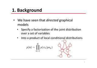
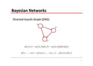
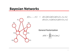
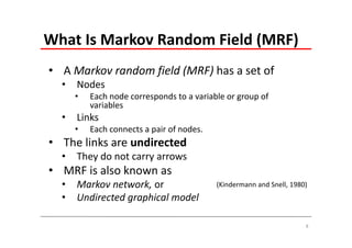
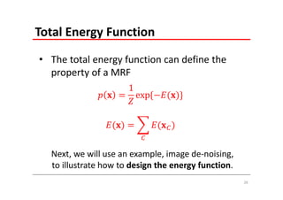
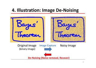
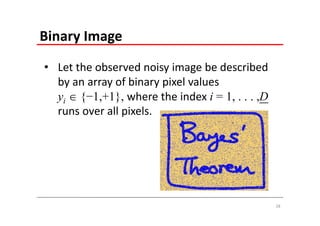
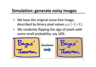
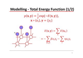
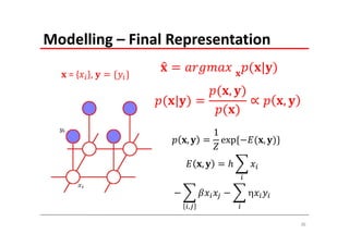
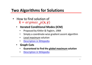
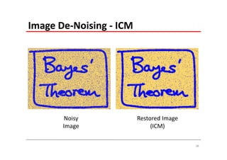
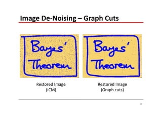
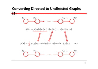
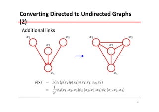
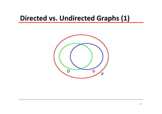
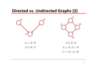
The document explains Markov Random Fields (MRFs) as a class of undirected graphical models used for modeling joint distributions and conditional independence properties, contrasting them with directed graphical models like Bayesian networks. It covers the factorization of joint distributions, the significance of energy functions in applications such as image de-noising, and the underlying relationships between directed and undirected graphs. Key concepts such as cliques, potential functions, and solution algorithms are also discussed.

1. Markov Random Field
Explained from the View of
Probabilistic Graphical Models
SUPPLEMENTS FOR
BAYESIAN NETWORKS COURSE
YUAN‐KAI WANG, 2011/05/05
1

2. Goal of This Unit
• We have seen that directed graphical models
specify a factorization of the joint distribution
over a set of variables into a product of local
conditional distributions
• We turn now to the second major class of
graphical models that are described by
undirected graphs and that again specify both
a factorization and a set of conditional
independence relations.
• We will talk Markov Random Field (MRF).
• No inference algorithms
• But more on modeling and energy function
2

3. Self‐Study Reference
• Source of this unit
• Section 8.3 Markov Random Fields, Pattern
Recognition and Machine Learning, C. M. Bishop,
2006.
• Background of this unit
• Chapter 8 Graphical Models, Pattern Recognition
and Machine Learning, C. M. Bishop, 2006.
• Probabilistic Graphical Models, Yuan‐Kai Wang’s
Lecture Notes for Bayesian Networks Courses,
2011.
3

4. Contents
1. Background
2. Conditional Independence Property
3. Factorization Property
4. Example: Image De‐noising
5. Relation to Directed Graphs
4

5. 1. Background
• We have seen that directed graphical
models
• Specify a factorization of the joint distribution
over a set of variables
• Into a product of local conditional distributions
5

6. Bayesian Networks
Directed Acyclic Graph (DAG)
6

7. Bayesian Networks
General Factorization
7

8. What Is Markov Random Field (MRF)
• A Markov random field (MRF) has a set of
• Nodes
• Each node corresponds to a variable or group of
variables
• Links
• Each connects a pair of nodes.
• The links are undirected
• They do not carry arrows
• MRF is also known as
• Markov network, or (Kindermann and Snell, 1980)
• Undirected graphical model
8

9. Why Use MRF for Computer Vision
• Image de‐noising
• Image de‐blurring
• Image segmentation
• Image super‐resolution
9

10. 2. Conditional Independence Property
• In the case of directed graphs, we can test
whether a conditional independence (CI)
property holds by applying a graphical test
called d‐separation.
• This involved testing whether or not the paths
connecting two sets of nodes were ‘blocked’.
• The CI definition will not apply to MRF and
undirected graphical models (UGMs).
• But we will find alternative semantics of CI
property for MRF and UGMs.
10

11. CI Definition for UGM
• Suppose that in an UGM we identify three
sets of nodes, denoted A, B, and C,
• And we consider the CI property
• To test whether CI property is satisfied by a
probability distribution defined by a UGM
• We consider all possible paths that connect
nodes in set A to nodes in set B through C.
11

12. An Example of CI
• Every path from any
node in set A to any
node in set B passes
through at least one
node in set C.
• Consequently the
conditional
independence property
holds for any probability
distribution described by
this graph.
12

13. Markov Blanket
• The Markov blanket for a UGM
takes a particularly simple form,
• Because a node will be conditionally
independent of all other nodes
Markov Blanket
conditioned only on the
neighbouring nodes.
13

14. 3. Factorization Property
• It is a factorization rule for UGM
corresponding to the conditional
independence test.
• What is factorization?
• Expressing the joint distribution p(x) as a
product of functions defined over sets of
variables that are local to the graph.
• Remember the factorization rule in directed
graphs Product of factors
14

15. The Factorization Rule – Two nodes
• Consider two nodes xi and xj that are not
connected by a link
• Then these variables must be conditionally
independent given all other nodes in the graph.
• There is no direct path between the two nodes.
• And all other paths pass through nodes that are
observed, and hence those paths are blocked.
• This CI property can be expressed as
x{i,j} denotes the set x of all variables with xi and xj removed.
15

16. The Factorization Rule – All Nodes
• Extend the factorization of two nodes to
the joint distribution p(x) of all nodes
• It must be the product of a set of factors
• Each factor has some nodes Xc={xi … xj} that do
not appear in other factors
• In order for the CI property to hold for all possible
distributions belonging to the graph.
,
16

17. Clique
,
• How to find the set of {xc}?
• We need to consider a graph terminology:
clique
• It is a subset of the nodes in a graph such that
there exists a link between all pairs of nodes in
the subset.
• The set of nodes in a clique is fully connected.
17

18. Cliques and Maximal Cliques
• A maximal clique is a clique that
• It is not possible to include any other nodes
from the graph to the set without it ceasing to
be a clique. Clique
Maximal Clique
18

19. An Example of Clique
• This graph has five cliques of two nodes
• {x1, x2}, {x2, x3}, {x3, x4}, {x4, x2}, {x1, x3}
• It has two maximal cliques Clique
• {x1, x2, x3}, {x2, x3, x4}
• The set {x1, x2, x3, x4} is
not a clique because of
the missing link
from x1 to x4.
Maximal Clique
19

20. Factorization by Maximal Clique
• We can define the factors in the
decomposition of the joint distribution to be
functions of the variables in the cliques.
,
• The set of nodes xC is a clique
• In fact, we can consider functions of the
maximal cliques, without loss of generality,
• Because other cliques must be subsets of maximal
cliques.
• The set of nodes xC is a maximal clique
20

21. The Factorization Rule
• Denote a clique by C and the set of
variables in that clique by xC.
• The joint distribution p(x) is written as a
product of potential functions C(xC) over
the maximal cliques of the graph
• The quantity Z, sometimes called partition
function, is a normalization constant and is
given by
21

22. Why Not Probability Function
for the Factorization Rule (1/2)
• Why potential function
but not probability function?
• In directed graphs, each factor represents the
conditional distribution corresponding to its
parents.
• But here we do not restrict the choice of
potential functions to a specific probabilistic
distribution.
22

23. Why Not Probability Function
for the Factorization Rule (2/2)
• Why potential function
but not probability function?
• It is all for flexibility
• We can define any function as we want
• But a little restriction (compared to probability)
has still to be made for potential function
C(xC).
• And note that the p(x) is still a probability
function
23

24. The Potential Function
• Potential function C(xC)
• C(xC)  0, to ensure that p(x)  0.
• Therefore it is usually convenient to express
them as exponentials
• E(xC) is called an energy function, and the
exponential representation is called the
Boltzmann distribution.
24

25. Energy Function
• The joint distribution is defined as the
product of potentials
• The total energy is obtained by adding the
energies of each of the maximal cliques.
1
ψ
1 1
exp exp
1
exp
25

26. Total Energy Function
• The total energy function can define the
property of a MRF
Next, we will use an example, image de‐noising,
to illustrate how to design the energy function.
26

27. 4. Illustration: Image De‐Noising
Original Image Image Capture Noisy Image
(binary image)
De‐Noising (Noise removal, Recover)
27

28. Binary Image
• Let the observed noisy image be described
by an array of binary pixel values
yi  {−1,+1}, where the index i = 1, . . . ,D
runs over all pixels.
28

29. Simulation: generate noisy images
• We have the original noise‐free image,
described by binary pixel values xi{−1,+1}.
• We randomly flipping the sign of pixels with
some small probability, say 10%.
Simulation
29

30. Modelling
• Because the noise level is small,
• There is a strong
correlation between
(noisy pixel)
xi and yi.
• We also know that
• Neighbouring pixels
xi and xj in an image
are strongly correlated.
xj
(noise‐free pixel)
30

31. Modelling ‐ Cliques
• This graph has two types of cliques, each of
which contains two variables.
• { xi , yi }
• { xi , xj }
• We need to define
two energy functions
for the two cliques.
xj
31

32. Modelling – Energy Function (1/2)
• { xi , yi } energy function
• Expresses the correlation
between these variables
• −xiyi
•  is a positive constant
• Why?
• Remember that
• A lower energy encouraging
a higher probability
• Low energy when xi and yi have the same sign
• Higher energy when they have the opposite sign
32

33. Modelling – Energy Function (2/2)
• { xi , xj } energy function
• Expresses the correlation
between these variables
• −xixj
•  is a positive constant xj
• Why?
• Low energy when xi and xj have the same sign
• Higher energy when they have the opposite sign.
33

34. Modelling ‐ Total Energy Function (1/2)
,
= { },

,
34

35. Modelling ‐ Total Energy Function (2/2)
• The complete energy function
for the model ,

(noisy pixel)
,
• We add an extra term hxi for each
pixel i in the noise‐free image.
• It has the effect of
• Biasing the model towards pixel
values that have one particular
(noise‐free pixel) sign in preference to the other
35

36. Modelling – Final Representation
= { },
1
, exp ,
,

,
36

37. Two Algorithms for Solutions
• How to find solution of
• Iterated Conditional Modes (ICM)
• Proposed by Kittler & Foglein, 1984
• Simply a coordinate‐wise gradient ascent algorithm
• Local maximum solution
• Description in Wikipedia
• Graph Cuts
• Guaranteed to find the global maximum solution
• Description in Wikipedia
37

38. Image De‐Noising ‐ ICM
Noisy Restored Image
Image (ICM)
38

39. Image De‐Noising – Graph Cuts
Restored Image Restored Image
(ICM) (Graph cuts)
39

40. 5. Relation to Directed Graphs
• We have introduced two graphical
frameworks for representing probability
distributions, corresponding to directed and
undirected graphs
• It is instructive to discuss the relation
between these.
• Details is TBU(To Be Updated)
40

41. Converting Directed to Undirected Graphs
(1)
41

42. Converting Directed to Undirected Graphs
(2)
Additional links
42

43. Directed vs. Undirected Graphs (1)
43

44. Directed vs. Undirected Graphs (2)
44