WC-H
WC-D
WC-U
2G-14 2G-15 2G-162G-172G-18 2G-19 2G-20 2G-21 2G-22 2G-23
2G-12
2G-13
2G-10
2G-11
2G-09
2G-08
2G-07
2G-06 2G-05
2G-04a
2G-04b
2G-03a
2G-03b
2G-02
2G-01a
2G-01b
2G-27
2G-26
2G-28
2G-29
2G-30
2G-31
2G-32
2G-33
2G-34
2G-35
2G-36
2G-37
2G-25
W.C.
2G-24a
2G-24b
2G-24c 2G-24d
2G-24e 2G-24f 2G-24g
2G-24h
2G-24i
2G-2Gl
2G-24m
2G-24n
2G-24p2G-24q2G-24r
2H-02
2H-03
2H-04
2H-05
2H-06
2H-07
2H-08
2H-09
2H-12
2H-13
2H-14
2H-15
2H-16
2H-17
2H-18
2H-19
2H-20
2H-102H-11
2H-29
2H-28
2H-27
2H-24
2H-23
2H-22 2H-21
2H-25
2H-26
111,00
118,20
111,00
118,50
118,50
118,30
115,00
115,00
114,90
EDIF. G-H - Q.118,30
Geom. G. C ar andente Geom. G. C ar andente
Geom. G. C ar andente
Geom. G. C ar andente Geom. G. C ar andente Geom. G. C ar andente
Geom. G. C ar andente
Geom. G. C ar andente
Geom. G. C ar andente
Geom. G. C ar andente
Geom. G. C ar andente
Geom. G.
Geom. G.
Geom. G. C ar andente
Geom. G.
Geom. G.
Geom. G. C ar andente
Geom. G. C ar andenteGeom. G. C ar andente
Geom. G. C ar andente Geom. G. C ar andente
Geom. G. C ar andente
Geom. G. C ar andente
Geom. G. C ar andente
Geom. G. C ar andente
Geom. G. C ar andente
Geom. G. C ar andente
Geom. G. C ar andente
Geom. G. C ar andente Geom. G. C ar andente
Geom. G. C ar andente
Geom. G. C ar andente
Geom. G. C ar andente
Geom. G. C ar andente
Geom. G. C ar andente
Geom. G. C ar andente
Geom. G. C ar andente
Geom. G. C ar andenteGeom. G. C ar andente Geom. G. C ar andenteGeom. G. C ar andente
Geom. G. C ar andenteGeom. G. C ar andente Geom. G. C ar andenteGeom. G. C ar andente
Geom. G. C ar andente
Geom. G. C ar andente
Geom. G. C ar andente Geom. G. C ar andente
Geom. G. C ar andente Geom. G. C ar andente Geom. G. C ar andente
Geom. G. C ar andenteGeom. G. C ar andente
Geom. G. C ar andente
Geom. G. C ar andente
Geom. G. C ar andente
Geom. G. C ar andente Geom. G. C ar andente
Geom. G. C ar andenteGeom. G. C ar andente
Geom. G. C ar andenteGeom. G. C ar andente
Geom. G. C ar andente
Geom. G. C ar andente
Geom. G. C ar andente Geom. G. C ar andente
Geom. G. C ar andente
Geom. G. C ar andente
Geom. G. C ar andente
Geom. G. C ar andente
Geom. G. C ar andente
Geom. G. C ar andente Geom. G. C ar andente Geom. G. C ar andente Geom. G. C ar andente
Geom. G. C ar andente Geom. G. C ar andenteGeom. G. C ar andente
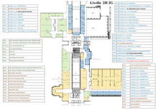
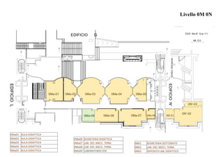
Livello 2H 2G
2H-01
2G-24
2H11 STUDIO (1 p) E. SANTAMATO
2H12 AMMINISTRAZIONE CNR/SPIN
2H13 STUDIO (1 p) C. Sciacca (prof. emerito)
2H14 STUDIO (1 p) A. ALOISIO
2H15 STUDIO (1 p) G. ABBATE
2H16 STUDIO (1 p) R. BRUZZESE
2H17 STUDIO (1 p) A. SASSO
2H18 STUDIO (1 p) L. LISTA (infn)
2H19 STUDIO (1 p) C. DE LISIO
2H20 STUDIO (2 p) G. RUSCIANO M. SALLUZZO (spin)
2H21 LAB. CALCOLO E ANALISI DATI FISICA SUBNUCLEARE
2H22 LAB. CALCOLO E ANALISI DATI FISICA SUBNUCLEARE
2H23/24 LAB. ATLAS/CMS/BELLE2
2H25 LAB. NA62/MURAVES
2H26 LAB. G-2
2H27 LAB. KM3
2H28 LAB. NEWS/SHIP/OPERA
2H29 LAB. NEWS/SHIP/OPERA
2G01 LAB. SPETTROSCOPIA LASER E MANIPOLAZIONE OTTICA
2G02 LAB. FISICA ATOMICA E APPLICAZIONI LASER
2G03a DIREZIONE CNR-SPIN
2G03b AMMINISTRAZIONE CNR-SPIN
2G04a UFFICIO PERSONALE INFN
2G04b SEGRETERIA DIREZIONE INFN
2G05 AMMINISTRAZIONE INFN
2G06 AMMINISTRAZIONE INFN
2G07 DIREZIONE INFN
2G08 DIREZIONE DIPARTIMENTO
2G09 AMMINISTRAZIONE DIPARTIMENTO
2G10 UFFICIO ACQUISTI DIPARTIMENTO
2G11 AMMINISTRAZIONE DIPARTIMENTO
2G12 UFFICIO MISSIONI DIPARTIMENTO
2G13 LAB. DIDATTICA DELLA FISICA
2G14 STUDIO (1 p) R. MASSA
2G15 STUDIO (1 p) L. CAMPAJOLA
2G16 STUDIO (1 p) G. ACAMPORA
2G17 STUDIO (1 p) A. ORDINE (infn)
2G18 STUDIO (1 p) G. OSTERIA (infn)
2G19 STUDIO (1 p) D. CAMPANA (infn)
2G20 STUDIO (1 p) E. VARDACI
2G21 STUDIO (1 p) A. GARGANO (infn)
2G22 STUDIO (1 p) D. PIERROTSAKOU (infn)
2G23 STUDIO (1 p) M. VIGILANTE
2G24 BIBLIOTECA DIPARTIMENTO
2G25 UFFICIO PROGETTI DIPARTIMENTO
2G26 SALA RIUNIONI
2G27 SALA RIUNIONI
2G28 STUDIO (1 p) E. CALLONI
2G29 STUDIO (1 p) P. RUSSO
2G30 STUDIO (1 p) L. DI FIORE (infn)
2G31 SALA RIUNIONI DIREZIONE
2G32 STUDIO (1 p) M.C. MONTESI, A. LAURIA
2G33 STUDIO (1 p) N. SPINELLI
2G34
STUDIO (2 p) M.R. MASULLO (infn), F.GALLUCCIO (infn),
C.GATTO (infn), V.G. Vaccaro (pensionato)
2G35 STUDIO (2 p) G. METTIVIER, P. MASSAROTTI
2G36 STUDIO (1 p) D. STORNAIUOLO
2G37 STUDIO (2 p) V. TATCHENKO (isasi), A. MARINO (isasi)
2H01 STUDIO (1 p) G. DE NARDO
2H02 STUDIO (2 p) G. MASTROIANNI (infn), M. IACOVACCI
2H03 STUDIO (1 p) M. Napolitano (prof. emerito)
2H04 STUDIO (1 p) T. DI GIROLAMO
2H05 STUDIO (1 p) G. DE LELLIS
2H06 STUDIO (1 p) G. BARBARINO
2H07 STUDIO (1 p) P. MIGLIOZZI (infn)
2H08 STUDIO (1 p) P. PAOLUCCI (infn)
2H09 STUDIO (2 p) M.G. ALVIGGI, G. CARLINO (infn)
2H10 STUDIO (1 p) L. MARRUCCI
2H11 STUDIO (1 p) E. SANTAMATO
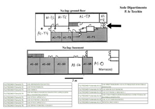
4.
0G-02/03
0G-01
OG-04
WC-H
WC-D
WC-U
1H-22b
1H-22a
1H.21a
1H-21b
1H-12b
1H-10
1H-08
1H-07
1H-09
1H-06
1H-05
1H-04
1H-03
1H-02d/e
1H-11b
1H-01
1G-01a
1G-01b
1G-01c
1G-01d 1G-02
1G-03b
1G-03a
1G-05
1G-06a
1G-06b
1G-07
1G-04
WC-D
WC-U
1G-09
1G-08
1G-10a
1G-19 1G-181G-17 1G-16 1G-15 1G-14 1G-13 1G-12
1G-11a
1G-20
1G-21
1G-22b
1G-22a
1G-23
1G-11b
1G-11b
1
2
EDIF. G-H - Q. 115,00
Geo m. G. Car an d en t e
Geo m. G. Car an d en t e
Geo m. G. Car an d en t e
Geo m. G. Car an d en t e
Geo m. G. Car an d en t e
Geo m. G. Car an d en t e
Geo m. G. Car an d en t e
Geo m. G. Car an d en t e
Geo m. G. Car an d en t e
Geo m. G. Car an d en t eGeo m. G. Car an d en t e
Geo m. G. Car an d en t e
Geo m. G. Car an d en t e
Geo m. G. Car an d en t eGeo m. G. Car an d en t e
Geo m. G. Car an d en t e
Geo m. G. Car an d en t e
Geo m. G. Car an d en t e
Geo m. G. Car an d en t e
Geo m. G. Car an d en t e
Geo m. G. Car an d en t e
Geo m. G. Car an d en t e
Geo m. G. Car an d en t e
Geo m. G. Car an d en t e
Geo m. G. Car an d en t e
Geo m. G. Car an d en t e
Geo m. G. Car an d en t e
Geo m. G. Car an d en t e
Geo m. G. Car an d en t e
Geo m. G. Car an d en t e
Geo m. G. Car an d en t e
Geo m. G. Car an d en t e Geo m. G. Car an d en t eGeo m. G. Car an d en t e
Geo m. G. Car an d en t e
Geo m. G. Car an d en t eGeo m. G. Car an d en t e Geo m. G. Car an d en t eGeo m. G. Car an d en t e
Geo m. G. Car an d en t eGeo m. G. Car an d en t eGeo m. G. Car an d en t eGeo m. G. Car an d en t e
Geo m. G. Car an d en t e
Geo m. G. Car an d en t e
Geo m. G. Car an d en t e
Geo m. G. Car an d en t e
Geo m. G. Car an d en t e
Geo m. G. Car an d en t e
Geo m. G. Car an d en t e
Geo m. G. Car an d en t eGeo m. G. Car an d en t e Geo m. G. Car an d en t eGeo m. G. Car an d en t e
Geo m. G. Car an d en t eGeo m. G. Car an d en t eGeo m. G. Car an d en t eGeo m. G. Car an d en t e
Geo m. G. Car an d en t eGeo m. G. Car an d en t e Geo m. G. Car an d en t eGeo m. G. Car an d en t e
Geo m. G. Car an d en t e Geo m. G. Car an d en t e Geo m. G. Car an d en t e Geo m. G. Car an d en t e
Geo m. G. Car an d en t e
Geo m. G. Car an d en t e
Geo m. G. Car an d en t e
Geo m. G. Car an d en t e Geo m. G. Car an d en t e
Geo m. G. Car an d en t e
Geo m. G. Car an d en t e
Geo m. G. Car an d en t e
Geo m. G. Car an d en t e
Geo m. G. Car an d en t eGeo m. G. Car an d en t e
Geo m. G. Car an d en t eGeo m. G. Car an d en t e
Geo m. G. Car an d en t e
Geo m. G. Car an d en t eGeo m. G. Car an d en t e
Geo m. G. Car an d en t eGeo m. G. Car an d en t e
Geo m. G. Car an d en t eGeo m. G. Car an d en t e
Geo m. G. Car an d en t eGeo m. G. Car an d en t e
Geo m. G. Car an d en t eGeo m. G. Car an d en t e
Geo m. G. Car an d en t e
Geo m. G. Car an d en t e
Geo m. G. Car an d en t e
Geo m. G. Car an d en t eGeo m. G. Car an d en t e
Geo m. G. Car an d en t e Geo m. G. Car an d en t e Geo m. G. Car an d en t e
Geo m. G. Car an d en t e
Geo m. G. Car an d en t e
Geo m. G. Car an d en t e
Geo m. G. Car an d en t e
Geo m. G. Car an d en t eGeo m. G. Car an d en t e
Geo m. G. Car an d en t eGeo m. G. Car an d en t eGeo m. G. Car an d en t e Geo m. G. Car an d en t e
Geo m. G. Car an d en t e
Geo m. G. Car an d en t e
Geo m. G. Car an d en t e
Geo m. G. Car an d en t eGeo m. G. Car an d en t e Geo m. G. Car an d en t e
Geo m. G. Car an d en t e
Geo m. G. Car an d en t e
Geo m. G. Car an d en t e
Geo m. G. Car an d en t e Geo m. G. Car an d en t e
Geo m. G. Car an d en t e
Geo m. G. Car an d en t e
Geo m. G. Car an d en t e Geo m. G. Car an d en t e
Geo m. G. Car an d en t e
Geo m. G. Car an d en t e
Geo m. G. Car an d en t e
Geo m. G. Car an d en t e
Geo m. G. Car an d en t eGeo m. G. Car an d en t e Geo m. G. Car an d en t e
Geo m. G. Car an d en t e
Geo m. G. Car an d en t e
Geo m. G. Car an d en t e
Geo m. G. Car an d en t eGeo m. G. Car an d en t e
Geo m. G. Car an d en t e Geo m. G. Car an d en t e
Geo m. G. Car an d en t e
Geo m. G. Car an d en t e
Geo m. G. Car an d en t e
Geo m. G. Car an d en t e
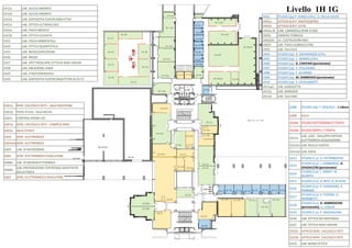
Livello 1H 1G
1H-01a1H-01b
1H-02a/b 1H-02c
1H-02f
1H-11a/c
1H-11d
1H- 12a
1H-24
1H-25
1H-26
1H-27
1H-28
1H-29
1H-30
1H-23
1G-01e
1G-10b
1H-22a
1H-21a
1H-22b
1H01 STUDIO (2p) P. IENGO (infn), D. DELLA VOLPE
1H01a UFFICIO SCR P. MASTROSERIO
1H01b UFFICIO SCR P. LO RE
1H02a /b LAB. LIMADOU/JEM-EUSO
1H02c CAMERA TERMICA
1H02d/e LA. COSTRUZIONI KM3
1H02f LAB. FISICA SUBNUCLEARE
1H03 LAB. Test Km3
1H04 STUDIO (1p) G. SEKHNIAIDZE (infn)
1H05 STUDIO (1p) C. ARAMO (infn)
1H06 STUDIO (1p) G. CHIEFARI (pensionato)
1H07 STUDIO (1p) V. PALLADINO
1H08 STUDIO (1p) F. GUARINO
1H09 STUDIO (1p) M. AMBROSIO (pensionato)
1H10 STUDIO (1p) S. CATALANOTTI
1H11a/c LAB. AUGER/CTA
1H11b LAB. DARKSIDE
1H11d LAB. Test KM3
1H12a LAB. SILICIO AMORFO
1H12b LAB. SILICIO AMORFO
1H21b LAB. DISPOSITIVI SUPERCONDUTTIVI
1H21a LAB. OTTICA ULTRAVELOCE
1H22a LAB. FISICA MEDICA
1H22b LAB. OTTICA GUIDATA
1H23 LAB. FISICA AMBIENTALE
1H24 LAB. OTTICA QUANTISTICA
1H25 LAB. NEWS/SHIP/OPERA
1H26 LAB. MODA
1H27 LAB. SPETTROSCOPIE OTTICHE NON LINEARI
1H28 LAB. ABLAZIONE LASER
1H29 LAB. STM/COHERENTIA
1H30 LAB. DISPOSITIVI SUPERCONDUTTORI ALTA TC
1G01a SERV. CALCOLO E RETI – SALA MACCHINE
1G01b TIER2 ATLAS - SALA RECAS
1G01c CONTROL ROOM LHC
1G01d SERV. CALCOLO E RETI – CAMPUS GRID
1G01e SALA UTENTI
1G02 SERV. ELETTRONICO
1G03a/b SERV. ELETTRONICO
1G04 LAB. DI MICROONDE
1G05 SERV. ELETTRONICO E RIVELATORI
1G06a LAB. DI MICROELETTRONICA
1G06b
LAB. PREPARAZIONE ESPERIENZE DIDATTICHE
DELLA FISICA
1G07 SERV. ELETTRONICO E RIVELATORI
1G08 STUDIO (2p) F. GESUELE + 1 Libero
1G09 AULA
1G10a STUDIO DOTTORANDI (7 POSTI)
1G10b STUDIO OSPITI ( 7 POSTI)
1G11a
LAB. LASS - SVILUPPO SISTEMI
ELETTRONICA ACQUISIZIONE
1G11b1 LAB. NUCLEI ESOTICI
1G11b2 LAB. EDEN
1G12 STUDIO (1 p) G. PATERNOSTER
1G13
STUDIO (2 p) I. LOMBARDO, G.
SPADACCINI (pensionato)
1G14
STUDIO (2 p) L. MANTI M.
QUARTO
1G15 STUDIO (2 p) A. BEST, A. DI LEVA
1G16
STUDIO (2 p) R. GIORDANO, A.
PORRINO
1G17
STUDIO (2 p) V. FERONE, G.
TROMBETTI
1G18
STUDIO (2 p) G. AMBROSONE
(pensionata), U. COSCIA
1G19 STUDIO (1 p) P. MADDALENA
1G20 LAB. OTTICA DEI MATERIALI
1G21 LAB. OTTICA NON LINEARE
1G22a UFFICIO SERV. CALCOLO E RETI
1G22b UFFICIO SERV. CALCOLO E RETI
1G23 LAB. NANO OTTICA
5.
0G-10
0G-09
OG-08
OG-11
OG-07
0G-12
WC
0G-02
0G-01
OG-04
0G-26
0G-27
0G-28
0G-25
0G-24
0G-13
0G-14
0G-15
0G-16
0G-17
0G-18
0G-19
0G-200G-210G-22
0G-23
WC-H
WC-D
WC-U
WC
111,00
111,00
111,70
111,00
108,30
110,65
110,70110,70
111,70
111,00
111,20
106,50
EDIF. G-H -Q. 111,70
Geom. G. C ar andente
Geom. G. C ar andenteG e om . G . Ca r a nde nte
G e om . G . Ca r a nde nte
Geom. G. C ar andente
Geom. G. C ar andente
Geom. G. C ar andente
Geom. G. C ar andente
Geom. G. C ar andente
G e om . G . Ca r a nde nte
Geom. G. C ar andente
Geom. G. C ar andente
Geom. G. C ar andente
Geom. G. C ar andente
Geom. G. C ar andenteGeom. G. C ar andente
Geom. G. C ar andente
Geom. G. C ar andenteGeom. G. C ar andente
G e om . G . Ca r a nde nteG e om . G . Ca r a nde nteGeom. G. C ar andente
Geom. G. C ar andente
Geom. G. C ar andente
Geom. G. C ar andente
Geom. G. C ar andente
Geom. G. C ar andente
G e om . G . Ca r a nde nte
Geom. G. C ar andente Geom. G. C ar andente Geom. G. C ar andente Geom. G. C ar andente Geom. G. C ar andente Geom. G. C ar andente
Geom. G. C ar andente
Geom. G. C ar andente Geom. G. C ar andente
Geom. G. C ar andenteGeom. G. C ar andente
Geom. G. C ar andente
Geom. G. C ar andente Geom. G. C ar andente
Geom. G. C ar andente Geom. G. C ar andente
Geom. G. C ar andente Geom. G. C ar andente
Geom. G. C ar andente
G e om . G . Ca r a nde nte
Geom. G. C ar andente
G e om . G . Ca r a nde nteG e om . G . Ca r a nde nte Geom. G. C ar andenteGeom. G. C ar andente
Geom. G. C ar andente
Geom. G. C ar andente
Geom. G. C ar andente
Geom. G. C ar andente Geom. G. C ar andente Geom. G. C ar andente
Geom. G. C ar andente
Geom. G. C ar andente Geom. G. C ar andente
Geom. G. C ar andente
Geom. G. C ar andente
Geom. G. C ar andente
Geom. G. C ar andente
Geom. G. C ar andenteGeom. G. C ar andente
Geom. G. C ar andenteGeom. G. C ar andente
Geom. G. C ar andente
Geom. G. C ar andente Geom. G. C ar andenteGeom. G. C ar andente
Geom. G. C ar andenteGeom. G. C ar andente
Geom. G. C ar andenteGeom. G. C ar andenteGeom. G. C ar andenteGeom. G. C ar andente
Geom. G. C ar andenteGeom. G. C ar andente
Geom. G. C ar andente
Geom. G. C ar andente
Geom. G. C ar andente
Geom. G. C ar andenteGeom. G. C ar andenteGeom. G. C ar andente
Geom. G. C ar andenteGeom. G. C ar andenteGeom. G. C ar andente
Geom. G. C ar andente
Geom. G. C ar andente Geom. G. C ar andente
Geom. G. C ar andenteGeom. G. C ar andente
Geom. G. C ar andenteGeom. G. C ar andenteGeom. G. C ar andenteGeom. G. C ar andente
Geom. G. C ar andente
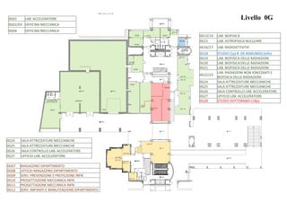
Livello 0G
0G22
0G23
0G21 0G20
0G24
0G25
0G26
0G27
OG-11
OG-12
0G01
0G02/03
0G04
0G01 LAB. ACCELERATORE
0G02/03 OFFICINA MECCANICA
0G04 OFFICINA MECCANICA
0G24 SALA ATTREZZATURE MECCANICHE
0G25 SALA ATTREZZATURE MECCANICHE
0G26 SALA CONTROLLO LAB. ACCELERATORE
0G27 UFFICIO LAB. ACCELERATORE
0G07 MAGAZZINO DIPARTIMENTO
0G08 UFFICIO MAGAZZINO DIPARTIMENTO
0G09 SERV. PREVENZIONE E PROTEZIONE INFN
0G10 PROGETTAZIONE MECCANICA INFN
0G11 PROGETTAZIONE MECCANICA INFN
0G12 SERV. IMPIANTI E MANUTENZIONE DIPARTIMENTO
0G13/14 LAB. BIOFISICA
0G15 LAB. ASTROFISICA NUCLEARE
0G16/17 LAB. RADIOATTIVITA’
0G18 STUDIO (1p) R. DE ASMUNDIS (infn)
0G19 LAB. BIOFISICA DELLE RADIAZIONI
0G20 LAB. BIOFISICA DELLE RADIAZIONI
0G21 LAB. BIOFISICA DELLE RADIAZIONI
0G22/23
LAB. RADIAZIONI NON IONIZZANTI E
BIOFISICA DELLE RADIAZIONI
0G24 SALA ATTREZZATURE MECCANICHE
0G25 SALA ATTREZZATURE MECCANICHE
0G26 SALA CONTROLLO LAB. ACCELERATORE
0G27 UFFICIO LAB. ACCELERATORE
0G28 STUDIO DOTTORANDI (18p)
6.
W.C.H.
M ONT ASCALE
MONT ASCALE
PUNTO RISTORO
Q.107.30
CAMERA BUIA
DEPOSITO
LABORATORIO
LOCALE DEPOSITO
LOCALE STUDENTI
SOTTOCENTRALE 5bis
Q.108.00
Q.107.30
Q.107.30
Q.107.30
Q.107.30
Q.107.30
Q.107.30
Q.107.30
Q.107.30
Q.107.30
Q.107.30
Q.107.30
Q.107.30
Q.107.30
Q.106.45
CUNICOLO
Q.106.45
ANT I W.C.
ANT I W.C.
Q.104.65
ST UDIO 1 ST UDIO 2 ST UDIO 3 ST UDIO 4 ST UDIO 5 ST UDIO 6
DEPOSIT O
Q.107.30
Q.104.65
M.CORPOA
Q.108.00 Q.108.40
Q.106.50
CUNICOLO Q.104.00
CAMMINAMENTO Q.108.40
Q.104.00
Q.105.30
Q.106.15
LOCALE COMPRESSORE
CENTRALE 5
TANDEM
W.C.H
W.C.
Q.106.15
Q.108.30
Q.105.70
Q.105.30
Q.105.30
CENTRALE ELETTRICA
Q.108.40
W.C.
W.C.
W.C.W.C.
W.C.
W.C.
W.C.
W.C.
-1G-04
-1G-06
-1G-07a
-1G-03
-1G-01g
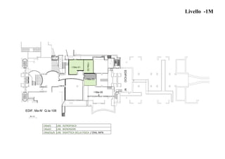
EDIF. G-H - Q. 107
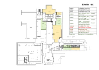
Livello -1G
-1G01h -1G01i
-1G-01f -1G-01e -1G-01a-1G-01b-1G-01c
-1G-01
-1G-01d
-1G-07b
-1G-05
-1G01a STANZA DITTA PULIZIE
-1G01b STANZA DITTA PULIZIE
-1G01c STANZA DITTA PULIZIE
-1G01d
LAB. FLUORESCENZA X - Locale
microscopi
-1G01e
LAB. FLUORESCENZA X - Sala
controllo Raggi X
-1G01f
LAB. FLUORESCENZA X - Locale
Raggi X (controllato)
-1G01h
LAB. FLUORESCENZA X - Locale
meccanica & chimica
-1G01g/i LAB. DIDATTICI O&O
-1G03 SALA STUDIO STUDENTI
-1G04 ex SALA MENSA
-1G05 ex DEPOSITO MENSA
-1G06 LAB. BIOFOTONICA
-1G07a/b LAB. SVILUPPI TECNOLOGICI
7.
2Ma-01
2Ma-02
2Ma-03 2Ma-04 2Ma-052Ma-06 2Ma-07 2Ma-08 2Ma-09 2Ma-10
2Ma-11
2MA-12
2Ma-22 2Ma-21 2Ma-20 2Ma-19 2Ma-18
2Ma-17
2Ma-16 2Ma-15
2Ma-14
2Ma-13
2Ma-23 2Ma-24 2Ma-25 2Ma-26 2Ma-27
2Ma-28
2Ma-29
2Ma-39 2Ma-38 2Ma-37 2Ma-36 2Ma-35 2Ma-34
2Ma-33 2Ma-32
2Ma-31
2Ma-30
2N'-01
2N'-02
2N'-03 2N'-04
2N'-05 2N'-06
2N'-22
2N'-21 2N'-20
2N'-07 2N'-08
2N'-09 2N'-10
2N'-11 2N'-12
2N'-19 2N'-18 2N'-17 2N'-16 2N'-15
2N'-13
2N'-23
2N'-442N'-45
2N'-24
2N'-25 2N'-26
2N'-27 2N'-28 2N'-29
2N'-43 2N'-42 2N'-41 2N'-40 2N'-39 2N'-38
2N'-37
2N'-36
2N'-35
2N'-342N'-33
2N'-322N'-31
2N'-30
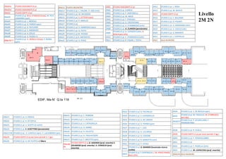
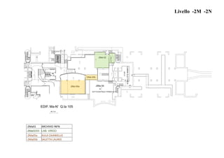
EDIF. Ma-N' Q.ta 118
Mt. 5.0
Q.E.
Livello
2M 2N
a
b
2Ma01a STUDIO ASSEGNISTI (4 p)
2Ma01b STUDIO ASSEGNISTI (5 p)
2Ma02 STUDIO OSPITI (3 p)
2Ma03
STUDIO (2 p) M.G. D’EMILIO (imaa), M. PICA
CIAMARRA (spin)
2Ma04 STUDIO (1 p) L. MEROLA
2Ma05 STUDIO (1 p) A. PORZIO (spin)
2Ma06 STUDIO (1 p) G. RICCIARDI
2Ma07 STUDIO (1 p) S. AMORUSO
2Ma08 STUDIO (1 p) A. ZOLLO
2Ma09 STUDIO (1 p) G. RUSSO ric.
2Ma10/11
STUDIO (2 p) A . BOSELLI (imaa), X. WANG
(spin)
2Ma12 PUNTO INCONTRO
2Ma13 STUDIO (2 p) L. VALORE, V. IZZO (infn)
2Ma14 STUDIO (1 p) M. NICODEMI
2Ma15 STUDIO (1 p) S. LETTIERI (isasi)
2Ma16 STUDIO (1 p) P. ANIELLO
2Ma17 STUDIO (1 p)
2Ma18 STUDIO (1 p) A. AMBROSIO (spin)
2Ma19 STUDIO (1 p) G. FESTA
2Ma20 STUDIO (1 p) M. PICOZZI
2Ma21 STUDIO (1 p) A. IMPARATO
2Ma22 STUDIO (1 p) G. PESCE
2N01 STUDIO ASSEGNISTI (2 p)
2N02 STUDIO (1 p) G.MIELE
2N03 STUDIO (1 p) P. SANTORELLI
2N04 STUDIO (1 p) M. ABUD
2N05 STUDIO (1 p) F. PERUGGI
2N06 STUDIO (1 p) G. CRISTOFANO
2N07 STUDIO (1 p) G. D’AMBROSIO (infn)
2N08 STUDIO (1 p) A. CLARIZIA (pensionato)
2N09
STUDIO (2 p) G. ESPOSITO (infn), G.
SCALA (aric infn)
2N10 STUDIO (1 p) C. STORNAIOLO (infn)
2N11 STUDIO (2 p) R. FIGARI, I. TESTA
2N12 STUDIO (1 p) L. ROSA
2N13 STUDIO (1 p) W. MUECK
2N15 STUDIO OSPITI (2 p)
2N16 STUDIO (1 p) E. BALZANO
2N17 STUDIO (1 p) O. PISANTI
2N18 STUDIO (1 p) G. MANGANO (infn)
2N19 STUDIO (1 p) A. COCCO (infn)
2N20 STUDIO (1 p) G. BIMONTE
2N21 STUDIO (1 p) L. CAPPIELLO
2N22 SALA RIUNIONE
2N23 STUDIO (1 p) B. PICCIRILLO
2N24 STUDIO (1 p) S. CAPOZZIELLO
2N25 STUDIO (1 p) A. DE CANDIA
2N26 STUDIO (1 p) A. FIERRO (spin)
2N27 STUDIO (1 p) F. LIZZI
2N28 STUDIO (1 p) A. LICCARDO
2N29 STUDIO (1 p) G. COVONE
2N30 STUDIO (1 p) R. MAROTTA (infn)
2N31 STUDIO (1 p) P. VITALE
2N32
STUDIO (1 p) G. MARMO (Incaricato ricerca
UniNA)
2N33
STUDIO (2 p) F.VENTRIGLIA, J. M. PEREZ PARDO
(bors infn)
2N34 STUDIO (1 p) S. DE NICOLA (spin)
2N35
STUDIO (2 p) M. PAOLILLO, M. D’ABRUSCO
(aric dip)
2N36/37
STUDIO (2 p) P. SCUDELLARO, F.
TRAMONTANO
2N38 STUDIO (1 p) R. FEDELE
2N39 STUDIO OSPITI (1 p) per brevi periodi (7 gg.)
2N40 STUDIO (1 p) E. PIEDIPALUMBO
2N41 STUDIO (1 p)
2N42 STUDIO (1 p) F. PEZZELLA (infn)
2N43 STUDIO (1 p) M. CAPACCIOLI (prof. emerito)
2N44/45 SALA RIUNIONI
2Ma23 STUDIO (1 p) A. EMOLO
2Ma24 STUDIO (1 p) R. DI CAPUA
2Ma25 STUDIO (1 p) U. SCOTTI DI UCCIO
2Ma26 STUDIO (1 p) E. SCHETTINO (pensionata)
2Ma27/28 STUDIO (2 p) G. CANTELE (spin) P. LUCIGNANO (spin)
2Ma29 STUDIO OSPITI (3 p) per brevi periodi (< 7 gg.)
2Ma30 STUDIO (2 p) G. DE FILIPPIS + 1 libero
2Ma31 STUDIO (1 p) C. PERRONI
2Ma32 STUDIO (1 p) C. ALTUCCI
2Ma33 STUDIO (1 p) V. CATAUDELLA
2Ma34 STUDIO (1 p) D. NINNO
2Ma35 STUDIO (1 p) R. VELOTTA
2Ma36 STUDIO (1 p) A. TAGLIACOZZO
2Ma37 STUDIO (1 p) F. MILETTO (spin)
2Ma38/
39
STUDIO OSPITI (3 p) G. IADONISI (prof. emerito) S.
SOLIMENO (prof. emerito) A. CONIGLIO (prof.
emerito)
8.
PASSERELLAMETALLICA
1Ma-01a
1Ma-01b
1Ma-02
1Ma-031Ma-04
1Ma-22 1Ma-21 1Ma-201Ma-19
1Ma-05 1Ma-06 1Ma-071Ma-08 1Ma-09
1Ma-10
1Ma-11 1Ma-12
1Ma-13 1Ma-14
1Ma-18
1Ma-17
1Ma-16
1Ma-15
1Ma-23 1Ma-24 1Ma-25 1Ma-261Ma-27
1Ma-28 1Ma-29
1Ma-30
1Ma-311Ma-32
1Ma-33
1Ma-34 1Ma-35
1Ma-36
1Ma-37
1Ma-38
1Ma-39
1N'-01
1N'-02a
1N'-02b 1N'-03 1N'-04
1N'-05
1N'-061N'-07
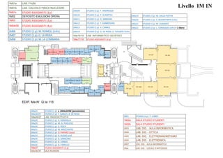
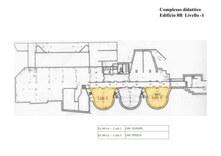
EDIF. Ma-N' Q.ta 115
Q.E.
Livello 1M 1N
1Ma23 STUDIO (1 p) L. SMALDONE (pensionato)
1Ma24/25 STUDIO (2 p) F. GARUFI, R. DE ROSA
1Ma26/27 LAB. RADIOATTIVITA’
1Ma28 STUDIO (1 p) A. RAMAGLIA
1Ma29 STUDIO (1 p) M. G. PUGLIESE
1Ma30 STUDIO (1 p) V. ROCA
1Ma31 STUDIO (1 p) M. MACCHIATO
1Ma32 STUDIO (1 p) D. PAPARO (isasi)
1Ma33 STUDIO (1 p) G. RUSSO prof.
1Ma34 STUDIO (1 p) G. SARACINO
1Ma35 STUDIO (1 p) G. LONGO
1Ma36 STUDIO (1 p) G. FIORILLO
1Ma37 STUDIO ASSEGNISTI (2 p)
1Ma38/39 SALA RIUNIONI
1N01 STUDIO (1 p) T. LERRO
1N02a SALA STUDIO STUDENTI
1N02b SALA STUDIO STUDENTI
1N03 LAB. DID. - AULA INFORMATICA
1N04 LAB. DID. - OTTICA
1N05 LAB. DID. - ELETTROMAGNETISMO
1N06 LAB. DID. - ELETTRONICA
1N07 LAB. DID. - AULA INFORMATICA
1Nxx LAB. DID. - LOCALE D’APPOGGIO
1Ma09 STUDIO (1 p) F. ANDREOZZI
1Ma10 STUDIO (1 p) P. SCAMPOLI
1Ma11 STUDIO (1 p) G. IMBRIANI
1Ma12 STUDIO (1 p) F. AMBROSINO
1Ma13 STUDIO (1 p) V. CANALE
1Ma14 STUDIO (2 p) G. DE ROSA, V. TIOUKOV (infn)
1Ma15/16 LAB. INFORMATICO GEOFISICI
1Ma17/18 STUDIO ASSEGNISTI (4 p)
1Ma19 STUDIO (1 p) M. DALLA PIETRA
1Ma20 STUDIO (1 p) S. BUONTEMPO (infn)
1Ma21 STUDIO (1 p) M. DURANTE
1Ma22 STUDIO (2 p) L. CORAGGIO (infn) + 1 libero
1M01a LAB. FAZIA
1M01b LAB. CALCOLO FISICA NUCLEARE
1M01c STUDIO ASSEGNISTI (2 p)
1M02 DEPOSITO EMULSIONI OPERA
1M03 STUDIO ASSEGNISTI (2 p)
1M04/05 STUDIO ASSEGNISTI (4 p)
1M06 STUDIO (1 p) M. ROMOLI (infn)
1M07 STUDIO (1 p) G. LA RANA
1M08 STUDIO (1 p) M. LA COMMARA
1Ma-01c